import torch
from torch import nn
from torch.utils.data import Dataset, DataLoader

# !pip install torchinfo if running in Colab
from torchinfo import summary

import pandas as pd
import numpy as np
import time

# for embedding visualization later
import plotly.express as px
import plotly.io as pio

# for appearance
pio.templates.default = "plotly_white"

# for train-test split
from sklearn.model_selection import train_test_split

# for suppressing bugged warnings from torchinfo
import warnings
warnings.filterwarnings("ignore", category = UserWarning)

# tokenizers from HuggingFace
from transformers import BertTokenizer

device = torch.device("cuda" if torch.cuda.is_available() else "cpu")18 Text Classification and Word Embedding
Open the live notebook in Google Colab or download the live notebook
.Major components of this set of lecture notes are based on the Text Classification tutorial from the PyTorch documentation.
To run this notebook in Google Colab, it is necessary to add the line !pip install torchinfo.
In this set of notes, we’ll discuss the problem of text classification. Text classification is a common problem in which we aim to classify pieces of text into different categories. These categories might be about:
- Subject matter: is this news article about news, fashion, finance?
- Emotional valence: is this tweet happy or sad? Excited or calm? This particular class of questions is so important that it has its own name: sentiment analysis.
- Automated content moderation: is this Facebook comment a possible instance of abuse or harassment? Is this Reddit thread promoting violence? Is this email spam?
We saw text classification previously when we first considered the problem of vectorizing pieces of text. We are now going to look at a somewhat more contemporary approach to text using word embeddings.
For this example, we are going to use a data set containing headlines from a large number of different news articles on the website HuffPost. I retrieved this data from Kaggle.
# access the data
url = "https://raw.githubusercontent.com/PhilChodrow/PIC16B/master/datasets/news/News_Category_Dataset_v2.json"
df  = pd.read_json(url, lines=True)
df  = df[["category", "headline"]]
There are over 200,000 headlines listed here, along with the category in which they appeared on the website.
df.head()| category | headline | |
|---|---|---|
| 0 | CRIME | There Were 2 Mass Shootings In Texas Last Week... |
| 1 | ENTERTAINMENT | Will Smith Joins Diplo And Nicky Jam For The 2... |
| 2 | ENTERTAINMENT | Hugh Grant Marries For The First Time At Age 57 |
| 3 | ENTERTAINMENT | Jim Carrey Blasts 'Castrato' Adam Schiff And D... |
| 4 | ENTERTAINMENT | Julianna Margulies Uses Donald Trump Poop Bags... |
Our task will be to teach an algorithm to classify headlines by predicting the category based on the text of the headline.
Training a model on this much text data can require a lot of time, so we are going to simplify the problem a little bit, by reducing the number of categories. Let’s take a look at which categories we have:
df.groupby("category").size()category
ARTS 1509
ARTS & CULTURE 1339
BLACK VOICES 4528
BUSINESS 5937
COLLEGE 1144
COMEDY 5175
CRIME 3405
CULTURE & ARTS 1030
DIVORCE 3426
EDUCATION 1004
ENTERTAINMENT 16058
ENVIRONMENT 1323
FIFTY 1401
FOOD & DRINK 6226
GOOD NEWS 1398
GREEN 2622
HEALTHY LIVING 6694
HOME & LIVING 4195
IMPACT 3459
LATINO VOICES 1129
MEDIA 2815
MONEY 1707
PARENTING 8677
PARENTS 3955
POLITICS 32739
QUEER VOICES 6314
RELIGION 2556
SCIENCE 2178
SPORTS 4884
STYLE 2254
STYLE & BEAUTY 9649
TASTE 2096
TECH 2082
THE WORLDPOST 3664
TRAVEL 9887
WEDDINGS 3651
WEIRD NEWS 2670
WELLNESS 17827
WOMEN 3490
WORLD NEWS 2177
WORLDPOST 2579
dtype: int64Some of these categories are a little odd:
- “Women”?
- “Weird News”?
- What’s the difference between “Style,” “Style & Beauty,” and “Taste”? ).
- “Parenting” vs. “Parents”?
- Etc?…
Well, there are definitely some questions here! Let’s just choose a few categories, and discard the rest. We’re going to give each of the categories an integer that we’ll use to encode the category in the target variable.
categories = {
    "STYLE"   : 0,
    "SCIENCE" : 1,
    "TECH" : 2,
}

df = df[df["category"].apply(lambda x: x in categories.keys())]
df.head()| category | headline | |
|---|---|---|
| 137 | TECH | Facebook Accused Of Reading Texts And Accessin... |
| 138 | TECH | Self-Driving Uber In Fatal Accident Had 6 Seco... |
| 155 | SCIENCE | Scientists Turn To DNA Technology To Search Fo... |
| 272 | TECH | Instagram Is Adding A 'Mute' Button For The Sa... |
| 285 | SCIENCE | Unusual Asteroid Could Be An Interstellar Gues... |
df["category"] = df["category"].apply(categories.get)
df| category | headline | |
|---|---|---|
| 137 | 2 | Facebook Accused Of Reading Texts And Accessin... |
| 138 | 2 | Self-Driving Uber In Fatal Accident Had 6 Seco... |
| 155 | 1 | Scientists Turn To DNA Technology To Search Fo... |
| 272 | 2 | Instagram Is Adding A 'Mute' Button For The Sa... |
| 285 | 1 | Unusual Asteroid Could Be An Interstellar Gues... |
| ... | ... | ... |
| 200844 | 2 | Google+ Now Open for Teens With Some Safeguards |
| 200845 | 2 | Web Wars |
| 200846 | 2 | First White House Chief Technology Officer, An... |
| 200847 | 2 | Watch The Top 9 YouTube Videos Of The Week |
| 200848 | 2 | RIM CEO Thorsten Heins' 'Significant' Plans Fo... |
6514 rows × 2 columns
The base rate on this problem is the proportion of the data set occupied by the largest label class:
df.groupby("category").size() / len(df)category
0 0.346024
1 0.334357
2 0.319619
dtype: float64If we always guessed category 1, then we would expect an accuracy of roughly 35%. So, our task is to see whether we can train a model to beat this. Towards this end, let’s perform a training-validation split.
df_train, df_val = train_test_split(df,shuffle = True, test_size = 0.2)Text Vectorization
Our next task is to vectorize the text headlines. One way to do this is one-hot encoding, in which we give each headline a feature for word w with value 1 if w appears in the headline. Today we’re going to do something a bit more aligned with modern practice. We’re going to use tokenization to break up each headline into a sequence of tokens, and then vectorize that sequence.
Tokenization starts with a tokenizer, which we import from HuggingFace.
tokenizer = BertTokenizer.from_pretrained("google-bert/bert-base-uncased")We can use this tokenizer like this:
tokenizer.tokenize("I love logistic regression!")['i', 'love', 'log', '##istic', 'regression', '!']For the purposes of modeling, it’s more convenient to assign an integer to each token, which we can do like this:
encoded = tokenizer("I love logistic regression!")
encoded
{'input_ids': [101, 1045, 2293, 8833, 6553, 26237, 999, 102], 'token_type_ids': [0, 0, 0, 0, 0, 0, 0, 0], 'attention_mask': [1, 1, 1, 1, 1, 1, 1, 1]}To undo this operation, we use the .decode method of the tokenizer:
tokenizer.decode(encoded["input_ids"])'[CLS] i love logistic regression! [SEP]'We’ll use this tokenizer to prepare a transformed version of our data set in consisting of the input_ids corresponding to each headline. We’ll write a preprocessing function which tokenizes each headline and then adds “padding” of 0s so that each tokenized headline has the same length.
X_train_tokenized = tokenizer(list(df_train["headline"]))["input_ids"]Our new training data is now a list of sequences of tokens. This list is “ragged” in the sense that the sequences are of different lengths. We can standardize the list by padding shorter sequences with 0s until all are the same length. We’ll use this preprocessing in the __init__() method of a torch Dataset class which will manage our data.
max_len = 50

def pad(l, max_len):
    assert len(l) <= max_len
    to_add = max_len - len(l)
    return l + [0]*to_add

def preprocess(df, tokenizer, max_len):
    X = tokenizer(list(df["headline"]))["input_ids"]
    X = [pad(t, max_len) for t in X]
    y = list(df["category"])
    return X, y

class TextDataFromDF(Dataset):
    def __init__(self, df):
        self.X, self.y = preprocess(df, tokenizer, 50)

    def __getitem__(self, ix):
        return self.X[ix], self.y[ix]

    def __len__(self):
        return len(self.y)
Now we can create datasets and data loaders from each of the training and validation data frames.
train_data = TextDataFromDF(df_train)
val_data   = TextDataFromDF(df_val)
A single piece of our data now looks like this:
X, y = train_data[1]
print(X)
print(y)
[101, 29500, 5329, 2907, 2061, 2172, 2769, 1996, 2194, 2071, 2022, 1037, 3054, 5332, 4371, 2924, 102, 0, 0, 0, 0, 0, 0, 0, 0, 0, 0, 0, 0, 0, 0, 0, 0, 0, 0, 0, 0, 0, 0, 0, 0, 0, 0, 0, 0, 0, 0, 0, 0, 0]
2To create data loaders, we need to define a collate_fn function which will accept a list of individual such X sequences and ensure that the result is a batch_size \(\times\) max_length sized 2d tensor.
def collate(data):
    X = torch.tensor([d[0] for d in data])
    y = torch.tensor([d[1] for d in data])
    return X,y

train_loader = DataLoader(train_data, batch_size=8, shuffle=True, collate_fn = collate)
val_loader = DataLoader(val_data, batch_size=8, shuffle=True, collate_fn = collate)
Let’s take a look at a batch of data now:
X, y = next(iter(train_loader))The predictor data is now a tensor in which the entries give token indices, padded with 0s. For visualization purposes we’ll show only the first 3 rows:
X[:3]tensor([[ 101, 2129, 2000, 2562, 2115, 4268, 1005, 2951, 3647, 3784,
102, 0, 0, 0, 0, 0, 0, 0, 0, 0,
0, 0, 0, 0, 0, 0, 0, 0, 0, 0,
0, 0, 0, 0, 0, 0, 0, 0, 0, 0,
0, 0, 0, 0, 0, 0, 0, 0, 0, 0],
[ 101, 9130, 10439, 3573, 1024, 1037, 12932, 3544, 102, 0,
0, 0, 0, 0, 0, 0, 0, 0, 0, 0,
0, 0, 0, 0, 0, 0, 0, 0, 0, 0,
0, 0, 0, 0, 0, 0, 0, 0, 0, 0,
0, 0, 0, 0, 0, 0, 0, 0, 0, 0],
[ 101, 1005, 2296, 2303, 2038, 1037, 2466, 1005, 21566, 4895,
8663, 27064, 2969, 1011, 2293, 102, 0, 0, 0, 0,
0, 0, 0, 0, 0, 0, 0, 0, 0, 0,
0, 0, 0, 0, 0, 0, 0, 0, 0, 0,
0, 0, 0, 0, 0, 0, 0, 0, 0, 0]])The target data is a tensor of integer indices:
y[:3]tensor([2, 2, 0])Modeling
Word Embedding
A word embedding refers to a representation of a word in a vector space. Each word is assigned an individual vector. The general aim of a word embedding is to create a representation such that words with related meanings are close to each other in a vector space, while words with different meanings are farther apart. One usually hopes for the directions connecting words to be meaningful as well. Here’s a nice diagram illustrating some of the general concepts:
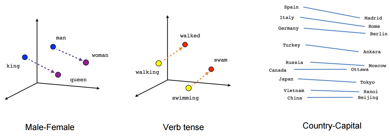
Image credit: Towards Data Science
Word embeddings are often produced as intermediate stages in many machine learning algorithms. In our case, we’re going to add an embedding layer at the very base of our model. We’ll allow the user to flexibly specify the number of dimensions.
We’ll typically expect pretty low-dimensional embeddings for this lecture, but state-of-the-art embeddings will typically have a much higher number of dimensions. For example, the Embedding Projector demo supplied by TensorFlow uses a default dimension of 200.
class TextClassificationModel(nn.Module):

    def __init__(self,vocab_size, embedding_dim, max_len, num_class):
        super().__init__()
        self.embedding = nn.Embedding(vocab_size+1, embedding_dim)
        self.fc   = nn.Linear(max_len*embedding_dim, num_class)

    def forward(self, x):
        x = self.embedding(x)
        x = torch.flatten(x, 1)
        x = self.fc(x)
        return(x)
Let’s learn and train a model!
vocab_size = len(tokenizer.vocab)
embedding_dim = 10
num_class = len(categories)

model = TextClassificationModel(vocab_size, embedding_dim, max_len, num_class).to(device)
summary(model, input_Size = (8, max_len))=================================================================
Layer (type:depth-idx) Param #
=================================================================
TextClassificationModel --
├─Embedding: 1-1 305,230
├─Linear: 1-2 1,503
=================================================================
Total params: 306,733
Trainable params: 306,733
Non-trainable params: 0
=================================================================optimizer = torch.optim.Adam(model.parameters(), lr=.1)
loss_fn = torch.nn.CrossEntropyLoss()
def train(dataloader):
epoch_start_time = time.time()
# keep track of some counts for measuring accuracy
total_acc, total_count = 0, 0
for X, y in dataloader:
# zero gradients
optimizer.zero_grad()
# form prediction on batch
predicted_label = model(X)
# evaluate loss on prediction
loss = loss_fn(predicted_label, y)
# compute gradient
loss.backward()
# take an optimization step
optimizer.step()
# for printing accuracy
total_acc += (predicted_label.argmax(1) == y).sum().item()
total_count += y.size(0)
print(f'| epoch {epoch:3d} | train accuracy {total_acc/total_count:8.3f} | time: {time.time() - epoch_start_time:5.2f}s')
def accuracy(dataloader):
total_acc, total_count = 0, 0
with torch.no_grad():
for X, y in dataloader:
predicted_label = model(X)
total_acc += (predicted_label.argmax(1) == y).sum().item()
total_count += y.size(0)
return total_acc/total_countEPOCHS = 20
for epoch in range(1, EPOCHS + 1):
train(train_loader)| epoch 1 | train accuracy 0.624 | time: 0.61s
| epoch 2 | train accuracy 0.875 | time: 0.48s
| epoch 3 | train accuracy 0.912 | time: 0.42s
| epoch 4 | train accuracy 0.952 | time: 0.57s
| epoch 5 | train accuracy 0.956 | time: 0.63s
| epoch 6 | train accuracy 0.974 | time: 0.52s
| epoch 7 | train accuracy 0.977 | time: 0.46s
| epoch 8 | train accuracy 0.983 | time: 0.46s
| epoch 9 | train accuracy 0.977 | time: 0.36s
| epoch 10 | train accuracy 0.984 | time: 0.54s
| epoch 11 | train accuracy 0.984 | time: 0.41s
| epoch 12 | train accuracy 0.990 | time: 0.42s
| epoch 13 | train accuracy 0.990 | time: 0.59s
| epoch 14 | train accuracy 0.988 | time: 0.54s
| epoch 15 | train accuracy 0.991 | time: 0.53s
| epoch 16 | train accuracy 0.993 | time: 0.49s
| epoch 17 | train accuracy 0.992 | time: 0.56s
| epoch 18 | train accuracy 0.991 | time: 0.47s
| epoch 19 | train accuracy 0.993 | time: 0.65s
| epoch 20 | train accuracy 0.993 | time: 0.55saccuracy(val_loader)0.8242517267843438Our accuracy on validation data is much lower than what we achieved on the training data. This is a possible sign of overfitting. Regardless, this predictive performance is much better than the roughly 34% that we would have achieved by guesswork:
Inspecting Word Embeddings
Recall from our discussion of image classification that the intermediate layers learned by the model can help us understand the representations that the model uses to construct its final outputs. In the case of word embeddings, we can simply extract this matrix from the corresponding layer of the model:
embedding_matrix = model.embedding.cpu().weight.data.numpy()Let’s also extract the words from our vocabulary:
tokens = list(tokenizer.vocab.keys())The embedding matrix itself has 3 columns, which is too many for us to conveniently visualize. So, instead we are going to use our friend PCA to extract a 2-dimensional representation that we can plot.
from sklearn.decomposition import PCA
pca = PCA(n_components=2)
weights = pca.fit_transform(embedding_matrix)
We’ll use the Plotly package to do the plotting. Plotly works best with dataframes:
tokens.append(" ")
embedding_df = pd.DataFrame({
    'word' : tokens,
    'x0'   : weights[:,0],
    'x1'   : weights[:,1]
})

embedding_df| word | x0 | x1 | |
|---|---|---|---|
| 0 | [PAD] | 1.801049 | 0.226354 |
| 1 | [unused0] | 1.167107 | 0.021828 |
| 2 | [unused1] | -0.902402 | -0.785311 |
| 3 | [unused2] | -0.952353 | 1.682580 |
| 4 | [unused3] | -1.381233 | -0.922989 |
| ... | ... | ... | ... |
| 30518 | ##/ | 0.002163 | -0.058429 |
| 30519 | ##: | -1.111538 | -0.144368 |
| 30520 | ##? | 0.000851 | -1.073678 |
| 30521 | ##~ | 0.123285 | 0.614450 |
| 30522 | 0.082506 | 0.211771 |
30523 rows × 3 columns
And, let’s plot! We’ve used Plotly for the interactivity: hover over a dot to see the word it corresponds to.
fig = px.scatter(embedding_df,
                 x = "x0",
                 y = "x1",
                 size = list(np.ones(len(embedding_df))),
                 size_max = 10,
                 hover_name = "word")

fig.show()
We’ve made an embedding! We might notice that this embedding appears to be a little bit “stretched out” in three main directions. Each one corresponds to one of the three classes in our training data.
Although modern methods for training word embeddings are much more complex, this example illustrates a key point: word embeddings are trained as byproducts of the process of training a model that learns to do something else, like text classification or predictive text generation.
Bias in Text Embeddings
Whenever we create a machine learning model that might conceivably have impact on the thoughts or actions of human beings, we have a responsibility to understand the limitations and biases of that model. Biases can enter into machine learning models through several routes, including the data used as well as choices made by the modeler along the way. For example, in our case:
- Data: we used data from a popular news source.
- Modeler choice: we only used data corresponding to a certain subset of labels.
With these considerations in mind, let’s see what kinds of words our model associates with female and male genders.
feminine = ["she", "her", "woman", "female"]
masculine = ["he", "him", "man", "male"]

highlight_1 = ["strong", "powerful", "smart",     "thinking", "brave", "muscle", "rough", "work"]
highlight_2 = ["hot",    "sexy",     "beautiful", "shopping", "children", "thin", "pretty", "home"]

def gender_mapper(x):
    if x in feminine:
        return 1
    elif x in masculine:
        return 4
    elif x in highlight_1:
        return 3
    elif x in highlight_2:
        return 2
    else:
        return 0

embedding_df["highlight"] = embedding_df["word"].apply(gender_mapper)
embedding_df["size"]      = np.array(1.0 + 50*(embedding_df["highlight"] > 0))

#
sub_df = embedding_df[embedding_df["highlight"] > 0]
import plotly.express as px
fig = px.scatter(sub_df,
x = "x0",
y = "x1",
color = "highlight",
size = list(sub_df["size"]),
size_max = 10,
hover_name = "word",
text = "word")
fig.update_traces(textposition='top center')
fig.update_layout(coloraxis_showscale=False)
fig.show()What do you notice about some of the similarities represented in these embeddings? What do you wonder?
Representational Harm and Representational Bias
Earlier in this course, we discussed allocative bias. Allocative bias occurs when different groups have inequitable opportunities to access important resources or opportunities on the basis of their identity. We discussed examples that raised questions about equitable access to personal liberty, employment, and insurance.
Representational bias refers to the systematic cultural representation of marginalized groups in harmful ways, or of denying them cultural representation at all. The perpetuation of harmful stereotypes is perhaps the most well-known form of representational harm. Erasure is another form of representational harm in which representations or topics of interest to marginalized groups are suppressed.
Here’s a very recent example (from Margaret Mitchell) illustrating how representational gender bias shows up in ChatGPT:
I replicated this (my screenshot below).
— MMitchell ((mmitchell_ai?)) April 23, 2023
Really great example of gender bias, for those of you who need a canonical example to make the point. https://t.co/O1A8Tk7oI1 pic.twitter.com/hKt4HSBzh3
Another form of representational harm in ML systems is the famous historical tendency of Google Search to surface demeaning and offensive search results related to people of color. This tendency was studied by Dr. Safiya Noble in her book Algorithms of Oppression. In one of Dr. Nobel’s most famous examples, top results for the phrase “black girls” in 2011 consisted of links to porn sites, which did not hold true of searches for “white girls” or “black men.” As late as 2016, an image search for “gorillas” would surface pictures of Black individuals. You can find a brief synopsis of some of Dr. Noble’s findings here (content warning: highly sexually explicit language). Google has since taken steps to improve these specific examples.
Bias in Google Translate
It is well-documented that machine learning algorithms trained on natural text can inherit biases present in those texts. One of the most direct ways in which we can observe such bias is in Google Translate. Some languages, such as Hungarian, do not possess gendered pronouns. When Google Translate attempts to render these pronouns into a gendered language like English, assumptions are made, as pointed out in this Tweet by Dora Vargha. Let’s demonstrate with the following English sentences.
he cooks. she is a political leader. she is an engineer. he is a cleaner. he is beautiful. she is strong.
Translate these into Hungarian and back via Google Translate, and here’s what you’ll get:
she cooks. he is a political leader. he is an engineer. she is cleaning. she is beautiful. he is strong.
Considering that English has a gender neutral pronoun (they), this would be an easy item to fix, which Google has thus far declined to do.
Intersections of Representational and Allocative Harms
In some cases, representational and allocative harms can intersect and reinforce each other. For example, modern translation systems perform impressively in certain languages but much less well in others. Some of these languages, such as Pashto and Dari, are spoken by many refugees and asylum-seekers to the US. The use of automated translation software when processing these asylum cases has drawn considerable scrutiny and appears to have resulted in the denial of at least one case due to a machine translation error.
More on Bias in Language Models
For more on the topic of bias in language models, you may wish to read the now-infamous paper by Emily Bender, Angelina McMillan-Major, Timnit Gebru, and “Shmargret Shmitchell” (Margaret Mitchell), “On the Dangers of Stochastic Parrots.” This is the paper that ultimately led to the firing of the final two authors by Google in late 2020 and early 2021.
© Phil Chodrow, 2025