So far in these notes, we have almost exclusively considered the classification problem: given some data with categorical labels, we aim to learn patterns in the data that will allow us to predict new labels for new unseen data. In the regression problem, we instead aim to learn patterns in the data that will allow us to predict a quantitative variable. If you want to predict the future price of a stock, the GPA of a Middlebury College student, or the number of wildfires in Vermont per year, you need to solve a regression problem.
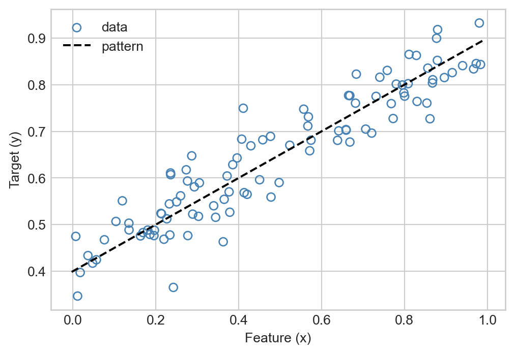
In these lecture notes we’ll focus on the linear regression problem and some of its extensions. Linear regression is an easy object of focus for us because it can be formulated in the framework of empirical risk minimization that we have recently been developing. In its most fundamental form, linear regression is the task of fitting a line to a cloud of points that display some kind of trend. Here’s the simple picture:
Code
import torchfrom matplotlib import pyplot as pltplt.style.use('seaborn-v0_8-whitegrid')def pad(x):return torch.cat([torch.ones(x.size(0), 1), x], dim =1)def regression_data(n =100, w = torch.Tensor([0.4, 0.5]), phi =lambda x: x, x_max =1): x = torch.rand(n, 1)*x_max x, ix = torch.sort(x) PHI = phi(x) PHI_ = pad(PHI) y = PHI_@w +0.05*torch.randn(n)return x, ydef plot_regression_data(X, y, w =None, phi =lambda x: x, pattern_label ="pattern", ax =None, legend =True, xlabel =True, ylabel =True, title =None):if ax isNone: fig, ax = plt.subplots(1, 1, figsize = (6, 4))if xlabel: labels = ax.set(xlabel ="Feature (x)")if ylabel: labels = ax.set(ylabel ="Target (y)")if title: t = ax.set(title = title) ax.scatter(X, y, facecolors ="none", edgecolors ="steelblue", label ="data")if w isnotNone: m_points =1001 x_ = torch.linspace(X.min().item()-0.01, X.max().item()+0.01, m_points) x_ = x_.reshape(-1, 1) PHI = phi(x_) PHI_ = pad(PHI) y_ = PHI_@w ax.plot(x_, y_, linestyle ="dashed", color ="black", label = pattern_label)if legend: ax.legend()return axw = torch.Tensor([0.4, 0.5])X, y = regression_data(w = w)plot_regression_data(X, y, w = w)
Our aim is to approximately learn the pattern when we are allowed only to observe the points.
Theoretically, linear regression is just another kind of empirical risk minimization. In practice, it has a few extra tricks.
Linear Regression as Empirical Risk Minimization
Consider the unregularized empirical risk minimization problem
Here, \(\ell\) is the per-observation loss function and \(\phi\) is a feature map. When studying convexity, we introduced several different choices of \(\ell\), including the 0-1 loss, logistic loss, and hinge loss.
Doing linear regression is as simple as choosing a different loss function. The most common choice is the square loss:
\[
\begin{aligned}
\ell(s, y) = (s - y)^2\;.
\end{aligned}
\]
Check that this per-observation loss function is convex as a function of \(s\).
With this choice, empirical risk minimization becomes least-squares linear regression, with loss function
The first term in this expression is the mean-squared error (MSE). Motivation via the MSE is the most common way that least-squares linear regression is motivated in statistics courses.
One can use the second-derivative test to check that the square loss is convex in \(s\), which means that all our standard theory from convex risk minimization translates to this setting as well. Gradient descent is one good method to learn the model and find \(\hat{\mathbf{w}}\), although there are many other good ways as well.
Matrix-Vector Formulation
It is possible to write Equation 11.2 much more simply using matrix-vector notation:
Here, \(\lVert \mathbf{v} \rVert_2^2 = \sum_{i}v_i^2\) is the squared Euclidean norm.
Using this gradient for a gradient-descent scheme would be a perfectly reasonable way to go about solving a least-squares linear regression problem.
Closed-Form Expression for Linear Regression
However, there is something special about least-squares linear regression: it’s actually not necessary to use gradient descent for small instances! Instead, we can solve the equation \(\nabla L(\hat{\mathbf{w}}) = \mathbf{0}\) directly. Starting from Equation 16.1, we can calculate
provided that the matrix inverse exists. This is a closed-form expression for the least-squares regression problem: no gradient descent required!
This computation, though simple to describe, is not necessarily easy. The matrix \(\mathbf{X}^T\mathbf{X}\) has dimensions \(p\times p\), where \(p\) is the number of features. When the number of features is very large, inverting this matrix may be computationally prohibitive.
Let’s implement this formula for linear regression as a simple class:
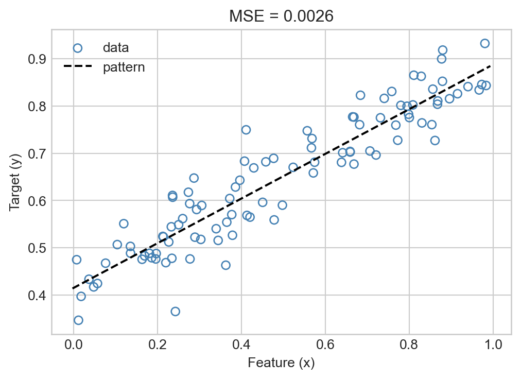
We can test this class on the data that we generated above, finding relatively good agreement with the data:
lr = LinearRegression()lr.fit(X, y)ax = plot_regression_data(X, y, w = lr.w)mse = lr.mse(X, y)title = ax.set(title =f"MSE = {mse:.4f}")
Linear Regression with Nonlinear Features
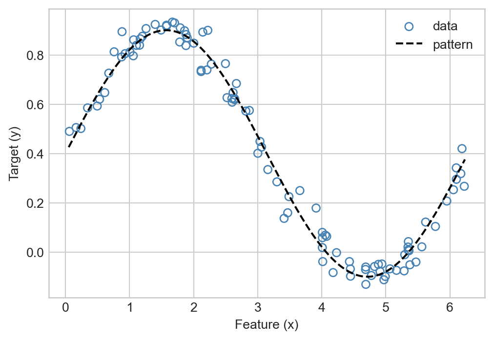
Suppose now that we wish to fit a regression model to some data that displays the following, nonlinear trend:
X, y = regression_data(100, w, x_max=2*torch.pi, phi = torch.sin)ax = plot_regression_data(X, y, w = w, phi = torch.sin)
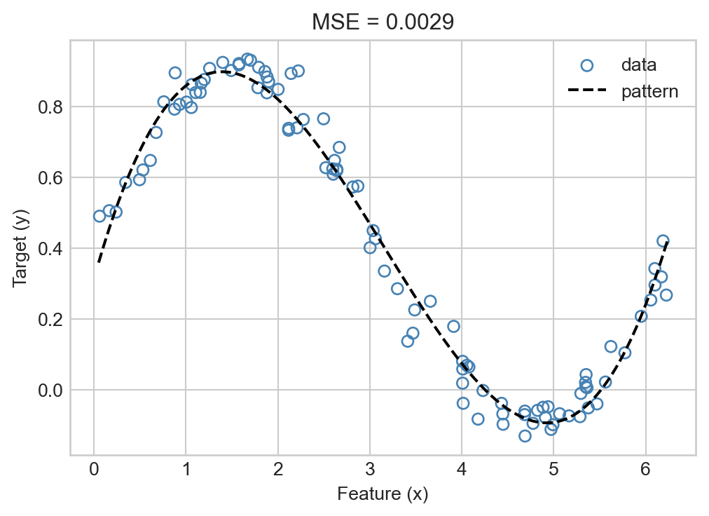
One way to approach this is via polynomial feature maps, which we’ve seen before. Since we’re using torch, we just need to define a helper function that outputs a tensor. We’re dropping the constant column added by the PolynomialFeatures since we add that back in as part of our model internals.
ax = plot_regression_data(X, y, w = lr.w, phi = phi)mse = lr.mse(PHI, y)title = ax.set(title =f"MSE = {mse:.4f}")
Predicting Health Costs
Let’s use our linear regression model to predict the cost of healthcare per patient. The data set we’ll use is from Obermeyer et al. (2019), which you may have encountered before. In this data set, each row corresponds to a patient. The data includes the gender, age, and race of the patient, as well as the results of various medical tests and other health-related characteristics.
import pandas as pdurl ="https://gitlab.com/labsysmed/dissecting-bias/-/raw/master/data/data_new.csv?inline=false"df = pd.read_csv(url)df = df.dropna() # remove rows that have missing data
For the purpose of our analysis today, we’ll discard the 1% of patients who had healthcare costs above $100,000. We’ll also consider only a subset of the columns in the data set, including a few selected medical features, age, gender, and race. We’ll also convert these into dummy columns.
df = df[df["cost_t"] <=100000]cols = [col for col in df.columns if"dem_age_band"in col and"18-24"notin col]cols += [col for col in df.columns if"elixhauser"in col]cols += [col for col in df.columns if"trig"in col]cols += ["dem_female", "race"]X_df = df[cols]X_df =1*pd.get_dummies(X_df, drop_first=True)col_names = X_df.columns # for laterX_df.head()
dem_age_band_25-34_tm1
dem_age_band_35-44_tm1
dem_age_band_45-54_tm1
dem_age_band_55-64_tm1
dem_age_band_65-74_tm1
dem_age_band_75+_tm1
alcohol_elixhauser_tm1
anemia_elixhauser_tm1
arrhythmia_elixhauser_tm1
arthritis_elixhauser_tm1
...
trig_min-high_tm1
trig_min-normal_tm1
trig_mean-low_tm1
trig_mean-high_tm1
trig_mean-normal_tm1
trig_max-low_tm1
trig_max-high_tm1
trig_max-normal_tm1
dem_female
race_white
1
0
0
1
0
0
0
0
0
1
0
...
0
1
0
0
1
0
0
1
1
1
8
0
1
0
0
0
0
0
0
0
0
...
0
1
1
0
1
1
0
1
1
0
15
0
0
0
0
1
0
0
0
0
0
...
0
0
0
0
0
0
0
0
1
1
19
0
1
0
0
0
0
0
0
0
0
...
0
1
0
0
1
0
0
1
0
1
21
0
0
0
0
0
1
0
0
0
0
...
0
1
0
0
1
0
0
1
1
1
5 rows × 41 columns
Now we can convert our feature data into a tensor. We’ll also construct a tensor holding the cost of medical care received by the patient.
X = torch.tensor(X_df.values, dtype=torch.float32)y = torch.tensor(df["cost_t"].values, dtype=torch.float32)
Finally, we’ll split the data into training and validation sets for model evaluation.
from sklearn.model_selection import train_test_splitX_train, X_val, y_train, y_val = train_test_split(X, y, test_size=0.2, random_state=802)
Let’s begin by calculating a baseline model performance. For this experiment, we’ll consider the baseline prediction to be the mean cost per patient:
The MSE of the baseline is quite high, indicating that different patients have very different amounts of healthcare spending. We’d like to achieve MSEs which are meaningfully lower than this on our validation set when modeling.
Let’s begin our modeling efforts by fitting a simple linear regression model:
lr = LinearRegression()lr.fit(X_train, y_train)lr_performance = lr.mse(X_val, y_val)print(lr_performance)
tensor(1.7944e+08)
This is already an improvement on the validation data! Can we do better? Maybe if we modeled some kind of nonlinear trend using polynomial features? To train and evaluate the model, we just need to construct the feature matrix by applying the feature map to the training and validation data.
_LinAlgError Traceback (most recent call last)File /Users/philchodrow/teaching/ml-notes/source/linear-regression.qmd:31 PHI_train = phi(X_train)2 lr = LinearRegression()---->3 lr.fit(PHI_train, y_train)Cell In[62], line 6462def fit(self, X, y):63 X_ = pad(X)--->64self.w = torch.inverse(X_.T@X_)@X_.T@y_LinAlgError: linalg.inv: The diagonal element 45is zero, the inversion could not be completed because the input matrix is singular.
The problem here is in the call torch.inverse(X_.T@X_) which is used in the fit method. According to the error, the matrix that we are trying to invert, \(\Phi(\mathbf{X})^T\Phi(\mathbf{X})\), is singular; i.e. the columns are linearly dependent. The reason this happens is that the polynomial feature map \(\Phi\) we’ve applied produces a lot of new columns. In fact, we face this issue in a lot of modern machine learning problems: we might have so many features that we don’t even know whether the data is linearly dependent or not. Simply applying linear regression according to Equation 11.5 will not work for such data sets. We can address this issue using regularization.
Ridge Regression
In ridge regression, we modify the empirical risk minimization problem Equation 11.2 by adding a regularization term to the loss function. The ridge-regularized empirical risk minimization problem is
The second term in this expression is the penalty term. We can see that this term is large when the entries \(w_{j}\) are large in magnitude. The effect of applying this term is therefore to shrink the entries of \(\mathbf{w}\) towards zero. The parameter \(\Lambda\) controls the strength of this effect: small values of \(\Lambda\) lead to results very similar to standard linear regression, while large values of \(\Lambda\) lead to very small values of \(\mathbf{w}\).
There is a small important subtlety in the regularization term in Equation 11.6: the sum over the entries of \(\mathbf{w}\) starts at \(j = 2\). We do this because the first entry of \(\mathbf{w}\), \(w_1\), corresponds to the constant feature and therefore corresponds to the overall scale of the data. Regularizing this term usually leads to systematic over- or under-estimation, and so we leave it out of the regularization term.
Fortunately, it’s possible to derive a closed-form expression for the ridge regression problem in a way which is very similar to regular linear regression. We can write the regularized empirical risk in matrix form as
where we’ve defined the matrix \[
\begin{aligned}
\mathbf{U} = \begin{pmatrix}
0 & \mathbf{0} \\
\mathbf{0} & \mathbf{I}
\end{pmatrix}
\end{aligned}
\]
with a \(0\) on the upper-left corner and the \((p-1)\times (p-1)\) identity matrix \(\mathbf{I}\) in the lower-right corner. The effect of multiplication by \(\mathbf{U}\) is to zero out the first entry of \(\mathbf{w}\), therefore excluding it from the regularization term.
Let’s construct a new class to implement ridge regression. We’ll let this class inherit from LinearRegression so that we can use the same methods for prediction and scoring.
class RidgeRegression(LinearRegression):def fit(self, X, y, lam =0.01): X_ = pad(X) n, p = X_.size(0), X_.size(1)# main computation U = torch.zeros(p, p) U[1:, 1:] = torch.eye(p-1)self.w = torch.inverse(X_.t()@X_ + lam*U)@X_.t()@y
Let’s go ahead and try out our ridge regression implementation:
This is already a modest improvement over the linear regression performance of tensor(1.7944e+08). Importantly, we can do even better with more features: it is possible to show that the matrix \(\Phi(\mathbf{X})^T\Phi(\mathbf{X}) + \lambda \mathbf{U}\) is invertible whenever \(\lambda > 0\). Let’s try the same computation as last time:
It’s also possible to train with even higher-dimensional feature maps, although this tends to make our computations slow (inverting large matrices is expensive) and is not guaranteed to lead to performance improvements.
Computational Complexity
Is that all there is to least-squares linear regression? Of course not!
Other Regularizers
Not if we use different regularization terms! An especially popular regularizer is the \(\ell_1\) regularizer, which penalizes entries of \(\mathbf{w}\) based on their absolute value rather than their square. If we use this regularizer in addition to or instead of the \(\ell_2\) regularization term, then we can’t use the closed-form matrix formula above.
Gradient Methods
More fundamentally, suppose that we have a very large number \(p\) of features. The matrix \(\Phi(\mathbf{X})^T\Phi(\mathbf{X}) + \lambda \mathbf{I}\) is a \(p\times p\) matrix. The computational cost of inverting this matrix is \(\Theta(n^\gamma)\) for some \(\gamma\) between \(2\) and \(3\). For sufficiently large \(p\), this may simply be infeasible. There are several approaches.
To perform gradient descent with least-squares linear regression, all we need is a formula for the gradient. Equation 16.1 gives this formula – we just plug in the gradient of the regularizing term and iterate to convergence.
Sometimes even this is too hard: for sufficiently large \(p\), even computing the matrix multiplication \(\Phi(\mathbf{X})^T\Phi(\mathbf{X})\) required for gradient descent is too computationally intensive. In this case, stochastic gradient methods can be used; we’ll study these in a coming lecture.
References
Obermeyer, Ziad, Brian Powers, Christine Vogeli, and Sendhil Mullainathan. 2019. “Dissecting Racial Bias in an Algorithm Used to Manage the Health of Populations.”Science 366 (6464): 447–53. https://doi.org/10.1126/science.aax2342.