Code
import torch
from matplotlib import pyplot as plt
import numpy as np
np.set_printoptions(precision = 3)
plt.style.use('seaborn-v0_8-whitegrid')Open the live notebook in Google Colab or download the live notebook
.Several times in these notes, we’ve encountered the problem of overfitting. Roughly, overfitting occurs when we choose a model that is too flexible or complex for the amount of data that we have available for training purposes. In this case, the model “fits the noise” instead of fitting the underlying pattern. The hallmark of overfitting is a model that performs well on the training data but much more poorly on test data.
In these notes, we’ll take a theoretical view of overfitting from the perspective of the bias-variance tradeoff in regression.
In any given machine learning problem, we are usually looking at a specific training set and a specific testing set. However, both these data sets are often random samples from a much larger set of possible data points. For this reason, we can also ask a question about the expected performance of a model on a sample from a data set:
If I generated many data sets in a similar way, trained models on those data sets, and then averaged over each, how good a prediction would I expect to make?
This is a theoretical way of asking how well we would expect a model to perform on a prediction task. As we’ll see, this way of asking the question will lead us to a helpful decomposition that lets us understand the sources of error in predictive modeling.
First, let’s visualize the kind of experiment we’re talking about here. We’ll generate some simple data for a regression task and then train a regression model on it multiple times. Here are a few runs:
import torch
from matplotlib import pyplot as plt
import numpy as np
np.set_printoptions(precision = 3)
plt.style.use('seaborn-v0_8-whitegrid')In this set of lecture notes, we’ll use the following bespoke implementation of least-squares linear regression with polynomial feature maps:
# polynomial feature map
def form_feature_matrix(x, order=1):
    X = torch.zeros((len(x), order+1))
    for i in range(0, order + 1):
        X[:,i] = x**i
    return X

# least squares linear regression
def find_pars(x, y, order=1):
    X = form_feature_matrix(x, order)
    w = torch.linalg.inv(X.T@X)@X.T@y
    return w

# predictor from learned parameters
def predict(x, w, order = 1):
    X = form_feature_matrix(x, order)
return X@wx = torch.linspace(-1, 1, 50)
# data generating process for the targets
# we're gonna keep the same predictors (x) throughout
def generate_data(x, w0, w1, sig = 0.4):
y = w0 + w1*x + 1*x**2 + 0.5*(x+1.2)*torch.normal(0, sig, size=x.shape)
return y
# plot some examples
fig, ax = plt.subplots(1, 3, figsize=(6.5, 2.5))
for i in range(3):
y = generate_data(x, 0, 1)
y_test = generate_data(x, 0, 1)
ax[i].scatter(x, y_test, alpha = 0.4, color = "firebrick")
y_hat = predict(x, find_pars(x, y))
ax[i].plot(x, y_hat, color='black')
ax[i].set(xlim = (-1, 1), ylim=(-1, 2), xlabel = r"$x$")
if i == 0:
ax[i].set(ylabel = r"$y$")
plt.tight_layout()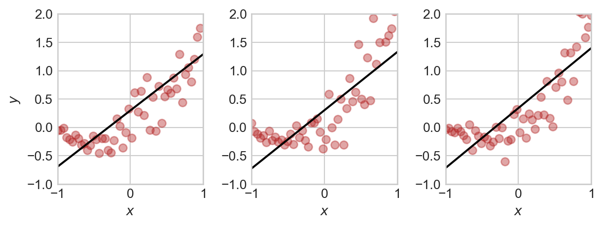
Note that, although each plot is similar, both the data set and the regression model that we learn from the data set are slightly different. This means that we’d get slightly different performance metrics each time.
In each repetition, we’ll save the targets and the predictions:
n_reps = 1000

targets = torch.zeros(n_reps, len(x))
predictions = torch.zeros(n_reps, len(x))

for i in range(n_reps):
    y = generate_data(x, 0, 1)
    y_hat = predict(x, find_pars(x, y))
    targets[i] = generate_data(x, 0, 1)
    predictions[i] = y_hat

mean_squared_error = torch.mean((targets - predictions)**2)

print(f"The average squared error per data point is {mean_squared_error:.2f}.")
The average squared error per data point is 0.17.Let’s look at the ensemble of models that we’ve produced:
fig, ax = plt.subplots(1, 1, figsize=(6, 4))

for i in range(n_reps):
    # ax.plot(x, targets[i], color='blue', alpha=0.1)
    ax.plot([x[0], x[-1]], [predictions[i,0], predictions[i,-1]], color='black', alpha=0.01)
    ax.set(xlabel = r"$x$", ylabel = r"$y$", title = "Ensemble of Linear Regression Models")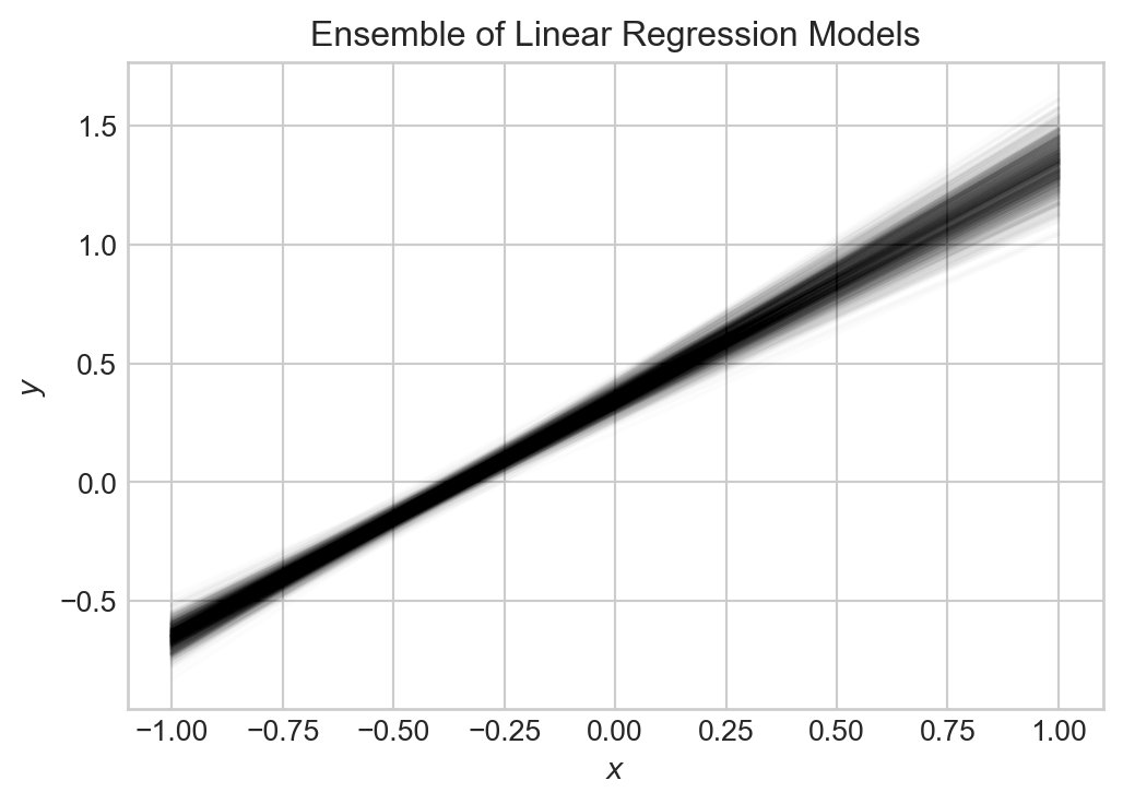
All of these models capture the general trend, but there is some variability. Indeed, in this framework, both the value of the target \(y\) at a point \(x_0\) and the value of our predictor \(\hat{y}\) at \(x_0\) are random variables. So, we can use tools from probability theory to analyze the mean-squared error, which we do now.
With some probability in hand, let’s return to our regression problem. Let’s consider just a single value of the predictor \(x_0\). In our repeated data generation experiment, the target at that predictor value in our training data is a random variable \(Y_t\). From this information (as well as the value of the training data at other predictor values), we obtain a predictor \(\hat{Y}\), which is a function of the training data.
Suppose now that we want to evaluate our predictor \(\hat{Y}\) against some testing data \(Y\). We think of \(Y\) as yet another random draw from the data generating distribution; it’s just one that we didn’t use to train our model. Because \(Y\) wasn’t used in the training of our model \(\hat{Y}\), we treat \(Y\) and \(\hat{Y}\) as independent random variables.
We want to know how well our predictor \(\hat{Y}\) is likely to do at predicting \(Y\) in a regression task. We’ll therefore consider the expected square loss at \(x_0\): \[ \begin{aligned} \mathcal{L}(x_0) = \mathbb{E}[(Y - \hat{Y})^2]\;, \end{aligned} \]
Here, the expectation is taken over the joint distribution of \(Y\) and \(\hat{Y}\). We can think of the expected square loss as a mathematical answer to the question we started with:
If I generated many data sets in a similar way, trained models on those data sets, and then averaged over each, how good a prediction would I expect to make?
We can get some insight on \(\mathcal{L}(x_0)\) with a bit of algebra. Let \(\mu = \mathbb{E}[Y]\) and \(\hat{\mu} = \mathbb{E}[\hat{Y}]\). Then, we can write the expected square loss into three terms:
\[ \begin{aligned} \mathcal{L}(x_0) &= \mathbb{E}[(Y - \hat{Y})^2] \\ &= \mathbb{E}[Y^2 - 2Y\hat{Y} + \hat{Y}^2] \\ &= \mathbb{E}[Y^2] - 2\mathbb{E}[Y\hat{Y}] + \mathbb{E}[\hat{Y}^2] \\ &= \mathbb{E}[Y^2] - 2\mathbb{E}[Y]\mathbb{E}[\hat{Y}] + \mathbb{E}[\hat{Y}^2] &\qquad \text{($Y$ and $\hat{Y}$ are independent)}\\ &= \mathbb{E}[Y^2] - 2\mu\hat{\mu} + \mathbb{E}[\hat{Y}^2] &\qquad \text{(def. of $\mu$ and $\hat{\mu}$)}\\ &= \mathbb{E}[Y^2] - \mu^2 + \mu^2 - 2\mu\hat{\mu} + \mathbb{E}[\hat{Y}^2] - \hat{\mu}^2 + \hat{\mu}^2 \\ &= \mathrm{var}(Y) + \mathrm{var}(\hat{Y}) + \mu^2 - 2\mu\hat{\mu} + \hat{\mu}^2 &\qquad \text{Variance formula}\\ &= \underbrace{\mathrm{var}(Y)}_{\text{noise}} + \underbrace{\mathrm{var}(\hat{Y})}_{\text{variance}} + \underbrace{(\mu - \hat{\mu})^2}_{\text{bias}} \\ \end{aligned} \]
Let’s take a moment with each of these terms.
Let’s compute each of these terms from the linear regression experiment that we did earlier. Since our analysis above was at a specific data point, we are going to compute values at each data point and then compare.
dim = 0 to each of these method calls ensures that the results for each data point are pooled separately.noise = targets.var(dim = 0, correction = 0)
variance = predictions.var(dim = 0, correction = 0)
bias = (targets.mean(dim = 0) - predictions.mean(dim = 0))**2
mse = ((targets - predictions)**2).mean(dim = 0)Now we can get a quantitative description of the sources of error in our model by plotting each one and the total mean-squared error. We’ll show this alongside an example data set and predictor for comparison:
fig, ax = plt.subplots(1, 2, figsize=(7, 3.5))

y = generate_data(x, 0, 1)
y_test = generate_data(x, 0, 1)
ax[0].scatter(x, y_test, alpha = 0.5, color = "firebrick")
y_hat = predict(x, find_pars(x, y))

ax[0].plot(x, y_hat, color='black')
ax[0].set(xlabel = r"$x$", ylabel = r"$y$", title = "Example data set and predictor")

ax[1].plot(x, noise, label = "data noise", linestyle = "--")
ax[1].plot(x, variance, label = "model variance", linestyle = "--")
ax[1].plot(x, bias, label = "model bias", linestyle = "--")
ax[1].plot(x, mse, label = "mse", color = "black")

ax[1].set(xlabel = r"$x$", ylabel = "Error", title =
"Bias-Variance Decomposition")

plt.legend()
plt.tight_layout()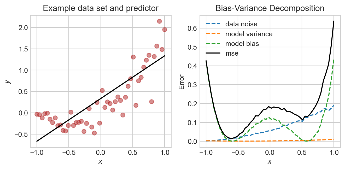
In this experiment, the noise and bias are the two primary contributors to the mean-squared error, with the model variance being quite low. The data generating process is deliberately constructed so that the data is noisier in certain regions, and so that the model bias also varies across regions.
In this particular case, we could likely achieve a better result by choosing a more flexible model with nonlinear features, as we’ll try soon.
If you were paying careful attention above, you may have noticed that increasing the model flexibility is a way to decrease bias but increase variance. This is the bias-variance tradeoff: often, reducing one of these two sources of error comes at the cost of increasing the other.
To illustrate the standard problem here, let’s run an experiment in which we train a series of polynomial regression models with increasing flexibility on a sinusoidal data set. Here are a few examples of the models we’ll train, with different orders:
def generate_sin_data(x, sig = 0.4):
    y = torch.sin(1*np.pi*x) + torch.normal(0, sig, size=x.shape)
    return y

fig, ax = plt.subplots(1, 2, figsize=(7, 3))

order = 1

y      = generate_sin_data(x)
y_test = generate_sin_data(x)

w     = find_pars(x, y, order)
y_hat = predict(x, w, order)

ax[0].scatter(x, y_test,  label = "data", color = "firebrick", alpha = 0.5)
ax[0].plot(x, y_hat, color='black', label = "model")
ax[0].set(title = f"Order {order}: Low Variance, High Bias", xlabel = r"$x$", ylabel = r"$y$")


order = 20
w     = find_pars(x, y, order)
y_hat = predict(x, w, order)

ax[1].scatter(x, y_test,  label = "data", color = "firebrick", alpha = 0.5)
ax[1].plot(x, y_hat, color='black', label = "model")
ax[1].set(title = f"Order {order}: Low Variance, High Bias", xlabel = r"$x$", ylabel = r"$y$")

plt.tight_layout()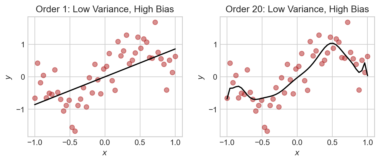
Now let’s estimate the terms in the bias-variance decomposition as we vary the model order:
fig, ax = plt.subplots(1, 1, figsize=(6, 4))

n_reps = 100
max_order = 10

variances = torch.zeros(max_order)
biases    = torch.zeros(max_order)
mses      = torch.zeros(max_order)
noises    = torch.zeros(max_order)

for order in range(0, max_order):

    targets = torch.zeros(n_reps, len(x))
    predictions = torch.zeros(n_reps, len(x))

    for i in range(n_reps):
        y = generate_sin_data(x)
        w = find_pars(x, y, order)
        y_hat = predict(x, w, order )
        targets[i] = generate_sin_data(x)
        predictions[i] = y_hat

    # noise of data
    noises[order] = targets.var(dim = 0, correction = 0).mean()

    # variance of predictions
    variances[order] = predictions.var(dim = 0, correction = 0).mean()

    # bias of predictions:
    biases[order] = ((targets.mean(dim = 0) - predictions.mean(dim = 0))**2).mean()

    mses[order] = ((targets - predictions)**2).mean()

ax.plot(torch.arange(max_order), mses, label = "mse", color = "black")
ax.plot(torch.arange(max_order), variances, label = "model variance", linestyle = "--")
ax.plot(torch.arange(max_order), noises, label = "data noise", linestyle = "--")
ax.plot(torch.arange(max_order), biases, label = "model bias", linestyle = "--")
ax.scatter(torch.arange(max_order), mses, color = "black")
ax.scatter(torch.arange(max_order), variances)
ax.scatter(torch.arange(max_order), noises)
ax.scatter(torch.arange(max_order), biases)


ax.set(xlabel = "Model Order", ylabel = "Error", title = "Illustration: Bias-Variance Tradeoff", xlim = (-0.5, None))

plt.legend()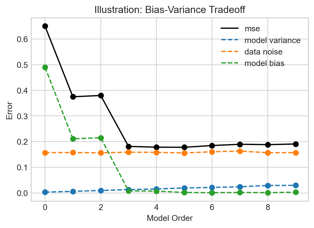
When the model order is small, the bias is very high – the model is underfit. As the model order increases, the bias shrinks rapidly, but the model variance begins to climb. Eventually, at order roughly 3, we reach a point at which the model is optimally flexible: increasing the model order will increase the model flexibility, and therefore variance, without enough of a benefit for reducing the bias.
It is also possible to observe the same bias-variance tradeoff by varying other hyperparameters that control the model flexibility, such as the regularization parameter \(\lambda\) in ridge regression.
The visualization in Figure 12.5 represents the classical view of the bias-variance tradeoff, and expresses the conventional wisdom of machine learning in roughly the era up until 2015 or so:
Adding more complexity to a model eventually becomes a bad idea.
The phenomenon in view here is sometimes called “single descent”: the MSE descends (once) as the model complexity increases, before increasing again past the optimal point.
However, this classical view leaves us with a mystery: if there is such a thing as too much model flexibility, then why is it that extremely flexible deep learning models with billions of parameters can perform well on data? In fact, in modern experiments we often observe a double descent phenomenon: the test error decreases with the model complexity, then increases, and then begins to decrease again:
The capability of highly-flexible models to avoid overfitting and achieve strong performance is a central insight of the deep learning revolution and an area of active research in the theory of machine learning.
In order to state the bias-variance tradeoff, we need to recall a few definitions from probability.
We provide the rapid review of definitions below for discrete sample spaces and random variables. The theory is not substantially different for continuous random variables, but the notation is more complicated.
Definition 12.1 (Sample Space and Events) A sample space \(S\) is a set of possible outcomes. An event \(A\) is a subset of the sample space \(S\). To each event \(A \subseteq S\) we can associate a probability \(\mathbb{P}(A)\) of the event occurring.
Definition 12.2 (Random Variables and Probability Mass Functions) A random variable \(X\) is a function that assigns a real number to each outcome in a sample space \(S\). The event \(X = x\) is the set of outcomes \(\{s \in S \;:\; X(s) = x\}\). The probability of the event \(X = x\) is \(\mathbb{P}(X = x)\). We often denote this probability as \(p_X(x)\). This function \(p_X\) is called the probability mass function of the random variable \(X\). We also often colloquially call it the “distribution” of \(X\).
Definition 12.3 (Jointly Random Variables, Marginals) Two random variables \(X\) and \(Y\) defined on the sample sample space \(S\) have a joint distribution \(p_{X,Y}(x, y) = \mathbb{P}(X = x \cap Y = y)\). The marginal distributions of \(X\) and \(Y\) are
\(p_X(x) = \sum_y p_{X,Y}(x, y)\) and \(p_Y(y) = \sum_x p_{X,Y}(x, y)\).
Definition 12.4 (Independence) Random variables \(X\) and \(Y\) are independent if it is the case that \(p_{X,Y}(x,y) = p_X(x)p_Y(y)\) for all \(x\) and \(y\).
Definition 12.5 (Expectation) The expectation of a random variable \(X\) is
\[ \begin{aligned} \mathbb{E}[X] = \sum_x x p_X(x). \end{aligned} \]
The expectation of a function of two jointly distributed random variables is
\[ \begin{aligned} \mathbb{E}[f(X,Y)] = \sum_{x,y} f(x,y) p_{X,Y}(x,y). \end{aligned} \]
Theorem 12.1 (Properties of the Expectation)
Definition 12.6 (Variance of a Random Variable) By definition, the variance of a random variable \(X\) is \(\mathrm{var}(X) = \mathbb{E}[(X - \mathbb{E}[X])^2]\).
A useful alternative formula for the variance is \(\mathrm{var}(X) = \mathbb{E}[X^2] - (\mathbb{E}[X])^2\).
© Phil Chodrow, 2025

.png)