import pandas as pd
import seaborn as sns
import numpy as np
from matplotlib import pyplot as plt
import matplotlib.cm as cm
sns.set_style("whitegrid")
np.set_printoptions(precision = 3)
pd.set_option('display.precision', 3)6 Statistical Definitions of Fairness in Decision-Making
Open the live notebook in Google Colab or download the live notebook
.In these notes, we’ll review three fundamental definitions of fairness for decision-making systems. While texts like Barocas, Hardt, and Narayanan (2023) couch their definitions in the language of probability, our focus in these notes will be to relate the formal mathematical language to operational computations on data sets in Python. In doing so, we’ll review some computational techniques via pandas, numpy, and seaborn from last time. After reviewing these definitions, we’ll review a simple, famous result about the ability of decision systems to satisfy multiple definitions.
For this study, we’ll return to the COMPAS data that we studied last time.
url = "https://raw.githubusercontent.com/PhilChodrow/ml-notes/main/data/compas/compas.csv"
compas = pd.read_csv(url)
For this discussion, we again only need to consider a subset of the columns, and we’ll focus exclusively on white (Caucasian) and Black (African-American) defendants:
cols = ["sex", "race", "decile_score", "two_year_recid"]
compas = compas[cols]

# using Angwin's definition
compas["predicted_high_risk"] = 1*(compas["decile_score"] > 4)

# subsetting by race
is_white = compas["race"] == "Caucasian"
is_black = compas["race"] == "African-American"

compas = compas[is_white | is_black]
compas = compas.copy()

# excerpt of the data

compas.head()| sex | race | decile_score | two_year_recid | predicted_high_risk | |
|---|---|---|---|---|---|
| 1 | Male | African-American | 3 | 1 | 0 |
| 2 | Male | African-American | 4 | 1 | 0 |
| 3 | Male | African-American | 8 | 0 | 1 |
| 6 | Male | Caucasian | 6 | 1 | 1 |
| 8 | Female | Caucasian | 1 | 0 | 0 |
Three Statistical Definitions of Fairness
Last time, we introduced the idea that fairness in decision-making could be defined formally, and models could be audited to determine the extent to which those models conformed to a given definition. In this section, we’ll discuss some of the definitions in Chapter 3 of Barocas, Hardt, and Narayanan (2023) and implement Python functions to measure the extent to which the COMPAS risk score conforms to those definitions.
To line ourselves up with the notation of Barocas, Hardt, and Narayanan (2023), let’s define the following random variables: Let \(A\) be a random variable that describes the group membership of an individual. Let \(Y\) be the outcome we want to predict. Let \(R\) be the value of our risk score. Let \(\hat{Y}\) be our model’s prediction about whether \(Y\) occurs.
In the case of COMPAS:
- \(A\) is the race of the individual, with possible values \(A = a\) and \(A = b\).
- \(Y = 1\) if the individual was arrested within two years after release, and \(Y = 0\) if not.
- \(R\) is the decile risk score.
- \(\hat{Y} = 1\) if \(R \geq 4\) and \(\hat{Y} = 0\) otherwise.
Statistical Independence
Here’s our first concept of fairness: independence. For our present purposes, we focus on the definition of independence for binary classifiers as given by Barocas, Hardt, and Narayanan (2023).
Definition 6.1 (Statistical Independence For Binary Classifiers) The model predictions \(\hat{Y}\) satisfy statistical independence if \(\mathbb{P}(\hat{Y} = 1 | A = a) = {P}(\hat{Y} = 1 | A = b)\).
Recall that \(\mathbb{P}(Y = 1|A = a)\) is the probability that \(Y = 1\) given that \(A=a\). It can be computed using the formula \(\mathbb{P}(Y = 1|A = a) = \frac{\mathbb{P}(Y = 1, A = a)}{\mathbb{P}(A = a)}\).
Colloquially, Definition 12.4 says that the probability of a positive prediction \(\hat{Y} = 1\) does not depend on the group membership \(A\). In the COMPAS data, independence would require that the probability of the model predicting that an individual will be arrested within two years be the same for Black and white defendants.
Let’s write a Python function to empirically check independence that will accept a data frame df and three additional arguments:
For independence, we don’t actually need the
target column, but this approach will let us keep a consistent API for our more complicated implementations below.group_col, the name of the column describing group memberships.target, the name of the column holding the binary outcomes.pred, the name of the column holding the predicted binary outcomes.
def test_independence(df, group_col, target, pred):
    out = df.groupby(group_col)[pred].agg(["mean", "size"])
    out.columns = ["positive prediction rate", "n"]
    return out.reset_index()
Let’s run our function to check for independence:
test_independence(compas, "race", "two_year_recid", "predicted_high_risk")| race | positive prediction rate | n | |
|---|---|---|---|
| 0 | African-American | 0.588 | 3696 |
| 1 | Caucasian | 0.348 | 2454 |
The mean column gives the proportion of the time in which the predictor \(\hat{Y}\) had value equal to 1, for each of the two groups. This is an empirical estimate of the probability \(\mathbb{P}(\hat{Y} = 1 | A = a)\). We can see that the two proportions are substantially different between groups, strongly suggesting that this model violates the independence criterion.
Formally, statistical tests beyond the scope of this course would be needed to reject the hypothesis that the two proportions are different. In this case, you can take my word for it that the relevant test provides strong support for rejecting the null.
As discussed in Barocas, Hardt, and Narayanan (2023), independence is a very strong expression of the idea that predictions, and therefore automated decisions, should be the same in aggregate across all groups present in the data. This idea sometimes accompanies another idea, that all groups are equally worthy, meritorious, or deserving of a given decision outcome.
Error-Rate Balance
The primary finding of Angwin et al. (2022) was, famously, that the COMPAS algorithm makes very different kinds of errors on Black and white defendants.
This definition can be generalized from binary classifiers to score functions via the concept of separation, which is discussed in Barocas, Hardt, and Narayanan (2023).
Definition 6.2 (Error Rate Balance for Binary Classifiers) The model predictions \(\hat{Y}\) satisfy error-rate balance if the following conditions both hold:
\[ \begin{aligned} \mathbb{P}(\hat{Y} = 1 | Y = 1, A = a) &= \mathbb{P}(\hat{Y} =1 | Y = 1, A = b) & \text{(balanced true positives)} \\ \mathbb{P}(\hat{Y} = 1 | Y = 0, A = a) &= \mathbb{P}(\hat{Y} =1 | Y = 0, A = b)\;. & \text{(balanced false positives)} \end{aligned} \]
Error rate balance requires that the true positive rate and false positive rates be equal on the two groups. Given some data in which we have \(\mathrm{TP}\) instances of true positives, \(\mathrm{FP}\) instances of false positives, \(\mathrm{TN}\) instances of true negatives, and \(\mathrm{FN}\) instances of false negatives, we can estimate the TPR and FPR via the formulas
\[ \begin{aligned} \mathrm{TPR} &= \frac{\mathrm{TP}}{\mathrm{TP} + \mathrm{FN}} \\ \mathrm{FPR} &= \frac{\mathrm{FP}}{\mathrm{FP} + \mathrm{TN}}\;. \end{aligned} \]
Let’s write another function with the same API to give a summary of error rates between two groups using these formulas. As we know, it’s pretty convenient to do this with confusion matrices. It’s not much more difficult to do it “by hand” using vectorized Pandas computations:
def test_error_rate_balance(df, group_col, target, pred):
    return df.groupby([group_col, target])[pred].mean().reset_index()
We can use this function to do an empirical test for error rate balance:
test_error_rate_balance(compas, "race", "two_year_recid", "predicted_high_risk")| race | two_year_recid | predicted_high_risk | |
|---|---|---|---|
| 0 | African-American | 0 | 0.448 |
| 1 | African-American | 1 | 0.720 |
| 2 | Caucasian | 0 | 0.235 |
| 3 | Caucasian | 1 | 0.523 |
The false positive rates are in the rows in which two_year_recid == 0, and the true positive rates are in the rows in which two_year_recid == 1.
As before, before concluding that the COMPAS algorithm violates error rate balance as in Definition 6.2, it is technically necessary to perform a statistical test to reject the null hypothesis that the true population error rates are the same.
Sufficiency
Finally, as we mentioned last time, the analysis of Angwin et al. (2022) received heavy pushback from Flores, Bechtel, and Lowenkamp (2016) and others, who argued that error rate balance wasn’t really the right thing to measure. Instead, we should check sufficiency, which we’ll define here for binary classifiers:
Definition 6.3 (Sufficiency) Model predictions \(\hat{Y}\) satisfy sufficiency if the following two conditions hold: \[ \begin{aligned} \mathbb{P}(Y = 1 | \hat{Y} = 1, A = a) &= \mathbb{P}(Y = 1 | \hat{Y} = 1, A = b) \\ \mathbb{P}(Y = 0 | \hat{Y} = 0, A = a) &= \mathbb{P}(Y = 0 | \hat{Y} = 0, A = b) \;. \end{aligned} \]
The quantity \(\mathbb{P}(Y = 1 | \hat{Y} = 1, A = a)\) is sometimes called the positive predictive value (PPV) of \(\hat{Y}\) for group \(a\). You can think of it as the “value” of a positive prediction: given that the prediction is positive (\(\hat{Y} = 1\)) for a member of group \(a\), how likely is it that the prediction is accurate? Similarly, \(\mathbb{P}(Y = 0 | \hat{Y} = 0, A = a)\) is sometimes called the negative predictive value (NPV) of \(\hat{Y}\) for group \(a\). So, the sufficiency criterion demands that the positive and negative predictive values be equal across groups.
Given some data in which we have \(\mathrm{TP}\) instances of true positives, \(\mathrm{FP}\) instances of false positives, \(\mathrm{TN}\) instances of true negatives, and \(\mathrm{FN}\) instances of false negatives, we can estimate the PPV and NPV via the formulas
\[ \begin{aligned} \mathrm{PPV} &= \frac{\mathrm{TP}}{\mathrm{TP} + \mathrm{FP}} \\ \mathrm{NPV} &= \frac{\mathrm{TN}}{\mathrm{TN} + \mathrm{FN}}\;. \end{aligned} \]
Let’s write a function to check for sufficiency in the COMPAS predictions. This function will compute the positive and negative predictive values by group:
def test_sufficiency(df, group_col, target, pred):
    df_ = df.copy()
    df_["correct"] = df_[pred] == df_[target]
    return df_.groupby([pred, group_col])["correct"].mean().reset_index()
test_sufficiency(compas, "race", "two_year_recid", "predicted_high_risk")| predicted_high_risk | race | correct | |
|---|---|---|---|
| 0 | 0 | African-American | 0.650 |
| 1 | 0 | Caucasian | 0.712 |
| 2 | 1 | African-American | 0.630 |
| 3 | 1 | Caucasian | 0.591 |
The negative predictive values are in the rows in which predicted_high_risk == 0 and the positive predictive values are in the rows in which predicted_high_risk == 1. We observe that the negative predictive value is slightly higher for white defendants, while the positive predictive value is slightly higher for Black defendants. These differences, however, are much lower than the error rate disparity noted above.
Can We Have It All?
Ok, well COMPAS isn’t an ideal algorithm by any means. But couldn’t we just define some more conceptions of fairness, pick the ones that we wanted to use, and then design an algorithm that satisfied all of them?
Sadly, no: we can’t even have error rate balance and sufficiency simultaneously.
Theorem 6.1 (Incompatibility of Error Rate Balance and Sufficiency (Chouldechova 2017)) If the true rates \(p_a\) and \(p_b\) of positive outcomes in the groups \(a\) and \(b\) are not equal (\(p_a \neq p_b\)), then there does not exist a model that produces predictions which satisfy both error rate balance and sufficiency.
Proof. Our big-picture approach is proof by contrapositive. We’ll show that if there were a model that satisfied error rate balance and sufficiency, then \(p_a = p_b\).
Let’s briefly forget about group labels – we’ll reintroduce them in a moment.
First, the prevalence of positive outcomes is the fraction of positive outcomes. There are \(\mathrm{TP} + \mathrm{FN}\) total positive outcomes, and \(\mathrm{TP} + \mathrm{FP} + \mathrm{TN} + \mathrm{FN}\) outcomes overal, so we can write the prevalence as
\[ \begin{aligned} p = \frac{\mathrm{TP} + \mathrm{FN}}{\mathrm{TP} + \mathrm{FP} + \mathrm{TN} + \mathrm{FN}};. \end{aligned} \]
From above, the true and false positive rates are:
\[ \begin{aligned} \mathrm{TPR} &= \frac{\mathrm{TP}}{\mathrm{TP} + \mathrm{FN}} \\ \mathrm{FPR} &= \frac{\mathrm{FP}}{\mathrm{FP} + \mathrm{TN}}\;. \end{aligned} \]
The PPV is: \[ \begin{aligned} \mathrm{PPV} = \frac{\mathrm{TP}}{\mathrm{TP} + \mathrm{FP}}\;. \end{aligned} \]
Ok, now it’s time to do some algebra. Let’s start with the \(\mathrm{TPR}\) and see if we can find an equation that relates it to the \(\mathrm{FPR}\). First, we’ll multiply by \(\frac{1 - \mathrm{PPV}}{\mathrm{PPV}}\). If we do this and insert the definitions of these quantities, we’ll get
\[ \begin{aligned} \mathrm{TPR} \frac{1 - \mathrm{PPV}}{\mathrm{PPV}} &= \frac{\mathrm{TP}}{\mathrm{TP} + \mathrm{FN}} \frac{\mathrm{FP}}{\mathrm{TP} + \mathrm{FP}} \frac{\mathrm{TP} + \mathrm{FP}}{\mathrm{TP}} \\ &= \frac{\mathrm{FP}}{\mathrm{TP} + \mathrm{FN}}\;. \end{aligned} \]
Let’s now also multiply by a factor of \(\frac{p}{1-p}\):
\[ \begin{aligned} \mathrm{TPR} \frac{1 - \mathrm{PPV}}{\mathrm{PPV}}\frac{p}{1-p} &= \frac{\mathrm{FP}}{\mathrm{TP} + \mathrm{FN}}\frac{p}{1-p} \\ &= \frac{\mathrm{FP}}{\mathrm{TP} + \mathrm{FN}} \frac{\mathrm{TP} + \mathrm{FN}}{\mathrm{TP} + \mathrm{FP} + \mathrm{TN} + \mathrm{FN}} \frac{\mathrm{TP} + \mathrm{FP} + \mathrm{TN} + \mathrm{FN}}{\mathrm{FP} + \mathrm{TN}} \\ &= \frac{\mathrm{FP}}{\mathrm{FP} + \mathrm{TN}} \\ &= \mathrm{FPR}\;. \end{aligned} \]
So, with some algebra, we have proven an equation for any classifier:
\[ \begin{aligned} \mathrm{TPR} \frac{1 - \mathrm{PPV}}{\mathrm{PPV}}\frac{p}{1-p} = \mathrm{FPR}\;. \end{aligned} \]
It’s convenient to rearrange this equation slightly:
\[ \begin{aligned} \frac{\mathrm{TPR}}{\mathrm{FPR}} \frac{1 - \mathrm{PPV}}{\mathrm{PPV}} = \frac{1-p}{p}\;. \end{aligned} \]
or
\[ \begin{aligned} p = \left(1 + \frac{\mathrm{TPR}}{\mathrm{FPR}} \frac{1 - \mathrm{PPV}}{\mathrm{PPV}}\right)^{-1}\;. \end{aligned} \tag{6.1}\]
Now suppose that I want to enforce error rate balance and sufficiency for two groups \(a\) and \(b\), where \(p_a \neq p_b\). So, from error rate balance I am going to require that \(\mathrm{TPR}_a = \mathrm{TPR}_b\), \(\mathrm{FPR}_a = \mathrm{FPR}_b\), and from sufficiency I am going to enforce that \(\mathrm{PPV}_a = \mathrm{PPV}_b\). Now, however, we have a problem: by Equation 6.1, it must also be the case that \(p_a = p_b\). This contradicts our assumption from the theorem. We cannot mathematically satisfy both error rate balance and sufficiency. This completes the proof.
The calculation above defines an inevitable tradeoff: if we want to ensure sufficiency when there are different prevalences between groups, then we will need to accept some amount of error rate imbalance. Similarly, if we want to ensure error rate balance, then we will need to accept some amount of disparity in sufficiency. There are a few ways to visualize this tradeoff. To start, let’s solve for the PPV in terms of the ratio between the TPR and FPR:
\[ \begin{aligned} \mathrm{PPV} = \frac{p \frac{\mathrm{TPR}}{\mathrm{FPR}}}{1-p + p \frac{\mathrm{TPR}}{\mathrm{FPR}}} \\ \end{aligned} \tag{6.2}\]
We can think of the ratio \(\frac{\mathrm{TPR}}{\mathrm{FPR}}\) as yet another compact measure of classifier quality: when this ratio is high, a positive prediction is a strong signal of a positive outcome. We can plot the PPV against this ratio:
Code
# gather various data for plot
error_rates = test_error_rate_balance(compas, "race", "two_year_recid", "predicted_high_risk")

tpr_fpr_ratio_black = error_rates.loc[1, "predicted_high_risk"] / error_rates.loc[0, "predicted_high_risk"]
tpr_fpr_ratio_white = error_rates.loc[3, "predicted_high_risk"] / error_rates.loc[2, "predicted_high_risk"]

sufficiency = test_sufficiency(compas, "race", "two_year_recid", "predicted_high_risk")

PPV_black = sufficiency.loc[2, "correct"]
PPV_white = sufficiency.loc[3, "correct"]

p = compas.groupby("race")["two_year_recid"].mean()
p_black = p.loc["African-American"]
p_white = p.loc["Caucasian"]

# construct plot

fig, ax = plt.subplots(1, 1, figsize = (5, 3.5))

tpr_fpr_ratio = np.linspace(0, 5, 100)

for i, p in enumerate([p_black, p_white]): # prevalences

    ppv = p*tpr_fpr_ratio/(1-p + p*tpr_fpr_ratio)

    ax.plot(tpr_fpr_ratio, ppv, color = cm.BuPu((i+.8)/2))


ax.set(ylim = (0, 1), )
plt.scatter(tpr_fpr_ratio_black, PPV_black, color = cm.BuPu((0+.8)/2), label = "Black defendants", zorder = 10)

hypothetical_ppv = p_white*tpr_fpr_ratio_black/(1-p_white + p_white*tpr_fpr_ratio_black)

plt.plot([tpr_fpr_ratio_black, tpr_fpr_ratio_black], [hypothetical_ppv, PPV_black], linestyle = "--", color = "black", linewidth = 1, zorder = 1)


hypothetical_tpr_fpr_ratio = 1.375


plt.scatter(tpr_fpr_ratio_white, PPV_white, color = cm.BuPu((i+.8)/2), label = "White defendants")

plt.plot([tpr_fpr_ratio_white, hypothetical_tpr_fpr_ratio], [PPV_white, PPV_white, ], linestyle = "--", color = "black", linewidth = 1, zorder = 1)

plt.legend()
ax.set(xlabel = "TPR/FPR", ylabel = "PPV")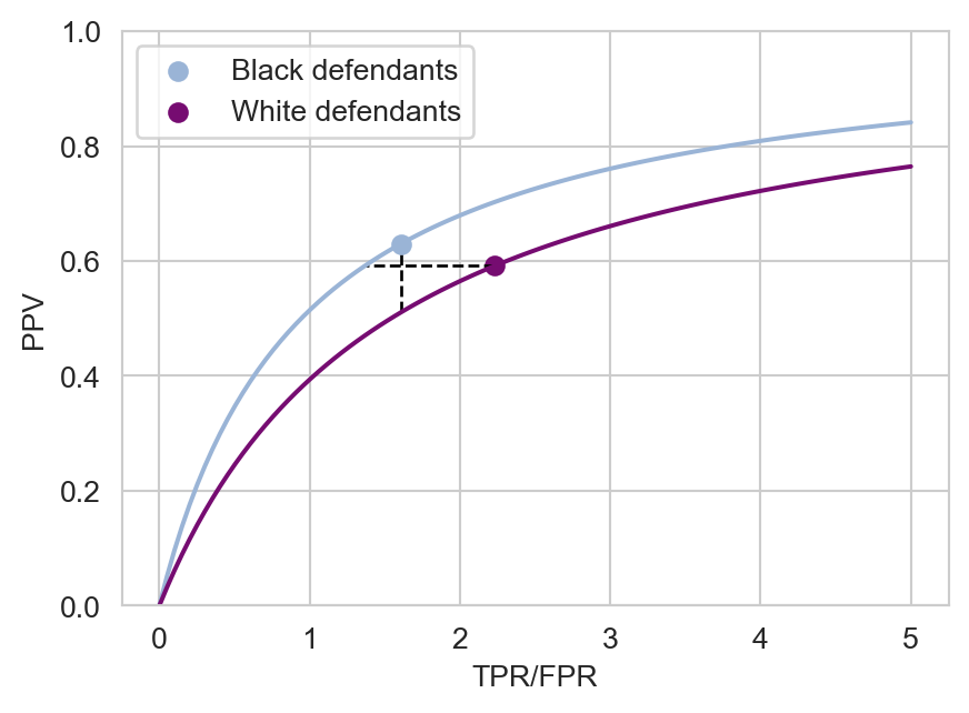
Figure 6.1 highlights the classifier design tradeoffs necessary to achieve either sufficiency or error rate balance. We’ve plotted the possible ratios between TPR and FPR on the horizontal axis and the corresponding possible PPVs on the vertical axis, all at the given prevalences among white and Black defendants, according to Equation 6.2. The solid points show the actual PPVs and TPR/FPR ratios for the COMPAS algorithm. Perfect sufficiency corresponds to each point being level with each other horizontally, while perfect error rate balance corresponds to each point being level with each other vertically. The fundamental difficulty is that we can’t move to the right and upward on these curves without access to better, more powerful classifiers, which usually requires more data. So, in order to achieve either of these criteria, we need to decrease classifier performance on at leaset one of the groups. We’ve visualized two options:
- To achieve sufficiency, we could slightly reduce both the TPR/FPR and the PPV on Black defendants, which would place their point at the end of the horizontal dashed line.
- To achieve error-rate balance, we could instead decrease both the TPR/FPR and the PPV on white defendants by a larger amount, which would place their point at the end of the vertical dashed line.
Both of these options highlight one of the fundamental difficulties of fairness in machine learning: can it really be the right thing to do to selectively decrease the predictive ability of a model on certain groups?
Fairness, Context, and Legitimacy
The proof above shows that, when the prevalences of positive outcomes differ between groups, we have no hope of being able to have both balanced error rates and sufficiency. In Chapter 3, Barocas, Hardt, and Narayanan (2023) give a few other examples of fairness definitions, as well as proofs that some of these definitions are incompatible with each other. We can’t just have it all – we have to choose.
The quantitative story of fairness in automated decision-making is not cut-and-dried – we need to make choices, which may be subject to politics. Let’s close this discussion with three increasingly difficult questions:
- What is the right definition of fairness by which to judge the operation of a decision-making algorithm?
- Is “fairness” even the right rubric for assessing the impact of a given algorithm?
- Is it legitimate to use automated decision-making at all for a given application context?
We’ll consider each of these questions soon.
References
Angwin, Julia, Jeff Larson, Surya Mattu, and Lauren Kirchner. 2022. “Machine Bias.” In Ethics of Data and Analytics, 254–64. Auerbach Publications.
Barocas, Solon, Moritz Hardt, and Arvind Narayanan. 2023. Fairness and Machine Learning: Limitations and Opportunities. Cambridge, Massachusetts: The MIT Press. https://fairmlbook.org/pdf/fairmlbook.pdf.
Chouldechova, Alexandra. 2017. “Fair Prediction with Disparate Impact: A Study of Bias in Recidivism Prediction Instruments.” Big Data 5 (2): 153–63. https://doi.org/10.1089/big.2016.0047.
Flores, Anthony W, Kristin Bechtel, and Christopher T Lowenkamp. 2016. “False Positives, False Negatives, and False Analyses: A Rejoinder to Machine Bias: There’s Software Used Across the Country to Predict Future Criminals. And It’s Biased Against Blacks.” Federal Probation 80: 38.
© Phil Chodrow, 2025