14 Some Practical Considerations

Data sets, transformations, and transfer learning.

Open the live notebook in Google Colab.

In this chapter, we continue our discussion of deep learning and consider some practical considerations for applied projects:

What should you do if your data is too large or otherwise inconvenient to hold in memory?
Can pre-trained models be used to speed up training and improve performance?
How can I match techniques to the kind of data that I have?

Code

import librosa
import pandas as pd
import numpy as np
import requests
from matplotlib import pyplot as plt
import os 
import torch
from torch.utils.data import Dataset, DataLoader
import warnings
from tqdm import TqdmWarning
warnings.filterwarnings("ignore", category=TqdmWarning)

!pip install torchinfo
from torchinfo import summary

zsh:1: /usr/local/bin/pip: bad interpreter: /usr/bin/python: no such file or directory
Requirement already satisfied: torchinfo in /Users/philchodrow/opt/anaconda3/envs/cs451/lib/python3.10/site-packages (1.8.0)

Audio Classification

We’ll explore a small audio classification task to illustrate some of these ideas. Our data set is a subset of the ESC-50 data prepared by Piczak (2015). This data set contains a total of 2000 audio files, each 5 seconds long, and labeled with one of 50 classes. Our task will be to predict the category of a sound based only on the audio.

Some of the categories not used in these lecture notes include “rain,” “crying baby,” “glass breaking,” “airplane,” and “crow.”

Figure 14.1: Example spectrograms from the ESC-50 data set. *Animation credit*: (Piczak 2015) at the associated GitHub repository.

First, we’ll download a dataframe containing the metadata for the audio files.

metadata_url = "https://raw.githubusercontent.com/karolpiczak/ESC-50/refs/heads/master/meta/esc50.csv"
metadata = pd.read_csv(metadata_url)
metadata.head()

	filename	fold	target	category	esc10	src_file	take
0	1-100032-A-0.wav	1	0	dog	True	100032	A
1	1-100038-A-14.wav	1	14	chirping_birds	False	100038	A
2	1-100210-A-36.wav	1	36	vacuum_cleaner	False	100210	A
3	1-100210-B-36.wav	1	36	vacuum_cleaner	False	100210	B
4	1-101296-A-19.wav	1	19	thunderstorm	False	101296	A

Importantly, we don’t yet have any audio files. This data frame contains information like the integer target label and the corresponding category name, and also includes train/test folds that the researchers constructed. Providing a metadata file like this one is helpful for large multimedia data. For example, it allows us to perform data subsetting and to organize our train/validation split before we download the data, which can be helpful for large data sets.

First, let’s pick a small number of categories to work with, and then we’ll download the corresponding audio files.

CATEGORIES = ["dog", "cow", "chirping_birds", "vacuum_cleaner"]
category_dict = {category: idx for idx, category in enumerate(CATEGORIES)}

metadata_subset = metadata[metadata["category"].isin(CATEGORIES)]
train_df = metadata_subset[metadata_subset["fold"] != 1]
val_df = metadata_subset[metadata_subset["fold"] == 1]

The resulting data sets are relatively small:

print(f"Number of training examples: {len(train_df)}")
print(f"Number of validation examples: {len(val_df)}")

Number of training examples: 128
Number of validation examples: 32

Now it’s time to actually access the audio files. Because we operated on the metadata first, we don’t have to download all 2,000 audio files from the repository directory; instead, we can just grab the ones we need. To illustrate working with data on filesystems, we’ll download the audio files and save them to disk.

The function below will download a single audio file and save it to the specified subdirectory of directory wav_data/, which will be created if necessary.

base_url = "https://github.com/karolpiczak/ESC-50/raw/refs/heads/master/audio"

def download_wav_data(wav_id, data_dir):
    
    # create a directory for each data set if it doesn't exist yet
    if not os.path.exists(f"wav_data/{data_dir}"):
        os.makedirs(f"wav_data/{data_dir}")
    
    # if the file isn't already downloaded, download it and save it to the appropriate directory
    destination = f"wav_data/{data_dir}/{wav_id}"
    if not os.path.exists(destination):
        url = f"{base_url}/{wav_id}"
        response = requests.get(url)
        with open(destination, "wb") as file:
            file.write(response.content)

We can now download the audio data by looping over the rows of each of our training and validation data frames. A simple syntactic alternative is to use the apply method of the data frame, which applies a function to each row of a specified column.

res = train_df["filename"].apply(lambda x: download_wav_data(x, "train"))
res = val_df["filename"].apply(lambda x: download_wav_data(x, "val"))

Let’s check that we’ve downloaded the data correctly:

num_training_files = len(os.listdir("wav_data/train"))
num_validation_files = len(os.listdir("wav_data/val"))

print(f"Number of training files: {num_training_files}")
print(f"Number of validation files: {num_validation_files}")

example_training_file = f"wav_data/train/{os.listdir('wav_data/train')[0]}"

print(f"Example training filename: {example_training_file}")

Number of training files: 128
Number of validation files: 32
Example training filename: wav_data/train/3-160993-A-3.wav

Looks good!

Waveforms and Spectrograms

I know very little about audio processing, so the discussion here is at a very low level of detail or expertise.

When we natively read in a .wav file, the result is an array describing a waveform:

waveform, sr = librosa.load(example_training_file, sr=16000)
print(type(waveform))
print(f"Shape of audio array: {waveform.shape}")
print(f"Sampling rate: {sr}")

<class 'numpy.ndarray'>
Shape of audio array: (80000,)
Sampling rate: 16000

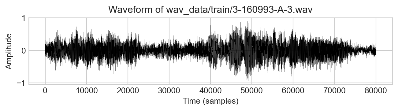
The sampling rate is 16,000 samples per second over 5 seconds, resulting in an array of 80,000 samples. The values in the array are floating point numbers between -1 and 1, which represent the amplitude of the sound wave at each sample:

Figure 14.2: Example waveform from the ESC-50 data set.

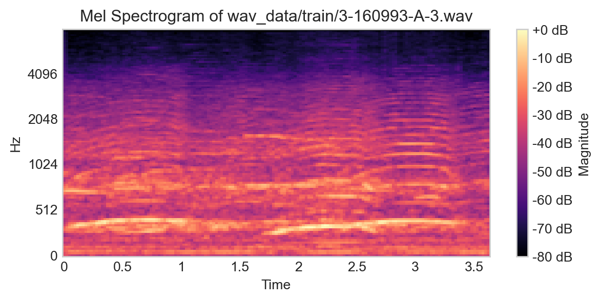
This waveform representation is, in principle, a perfectly valid input to a classification model, and contains 80,000 features. However, there are other representations of audio files which are also often useful. One of these is the spectrogram, which is a 2D representation of the audio file that captures how the frequency content of the sound changes over time. A common variant of the spectrogram is the Mel spectrogram, which uses a particular nonlinear transformation of the frequency axis to better capture human perception of sound.

Spectrograms are computed via Fourier transforms, in modern contexts usually the “fast Fourier transform (FFT).”

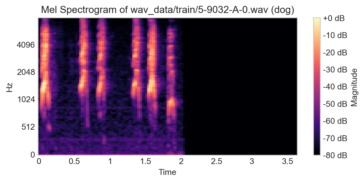
Figure 14.3: Example Mel spectrogram for a single training example.

Data From Filesystems

Now that we’ve seen two ways of representing the raw audio data, how are we going to feed this data into a model? Ideally, we’d like to do this in a way that (a) doesn’t require storing all the data in memory and (b) allows us to experiment with different data representations (e.g. waveform vs. spectrogram) and model architectures.

The key idea here is to implement an abstract DataSet with functionality for returning and optionally transforming data. The backend work is primarily to implement a __getitem__ method that supplies the user with a single data point at a time, including features, the target value, and any other desired metadata (such as the class names). This allows us to abstract away the handling of the filesystem from the user and makes it much easier to perform experiments.

We’ll also let the Dataset class handle determining the device on which the data should live, so first we need to discern the device:

device = "cuda" if torch.cuda.is_available() else "cpu"
print(f"Running on {device}.")

Running on cpu.

Now we implement the Dataset class.

class WavDataset(Dataset):
    def __init__(self, metadata, path, transform=None):
1        self.metadata = metadata
2        self.transform = transform
3        self.path = path

    def __len__(self):
4        return len(self.metadata)

    def __getitem__(self, idx):

        # figure out which filename corresponds to the 
        # specified index in self.metadata
        wav_id = self.metadata.iloc[idx]["filename"] 
        wav_path = f"wav_data/{self.path}/{wav_id}"

        # corresponding target value
5        label = self.metadata.iloc[idx]["category"]
6        category = category_dict[label]
        # load in the audio
        audio, sr = librosa.load(wav_path, sr=16000)
        if self.transform:
            audio = self.transform(audio)
        
        audio = torch.tensor(audio, dtype=torch.float32)
        category = torch.tensor(category, dtype=torch.long)

        return audio.to(device), category.to(device), label

1: Save the metadata dataframe for use in the __len__ and __getitem__ methods.
2: Save an optional transform function that can be applied to the raw audio data, for example a pipeline for computing the spectrogram.
3: Save the path to the data (e.g. “train” or “val”) for use in constructing the path to the audio files.
4: The length of the data set is just the number of rows in the metadata data frame.
5: The target label is the string in the category column of the metadata data frame.
6: The category is the integer value corresponding to the label, which we can get from the category_dict dictionary.

Since we are ultimately going to predict the category (target) from the audio, we need to move both of these to the device. The label is just for visualization purposes and won’t actually be used in a model.

Let’s try creating our training and validation data sets:

train_dataset = WavDataset(train_df, "train")
val_dataset   = WavDataset(val_df, "val")

Because we implemented __len__ and __getitem__, we can do things like this:

audio, category, label = train_dataset[0]

print(f"Shape of audio (features): {audio.shape}")
print(f"Category integer: {category}")
print(f"Category label: {label}")

print(f"Total number of training examples: {len(train_dataset)}")

Shape of audio (features): torch.Size([80000])
Category integer: 1
Category label: cow
Total number of training examples: 128

Datasets are also effortlessly compatible with DataLoaders, which means we can set ourselves up for a stochastic training loop with minimal additional effort:

train_loader = DataLoader(train_dataset, batch_size=8, shuffle=True)
val_loader   = DataLoader(val_dataset, batch_size=8, shuffle=False)

Flexible Data Sets

The flexibility of the dataset interface allows us to do the work once of defining a dataset, after which we can work with with code as simple as we would write for a data set held in memory. The interface even allows us greater flexibility. For example, we could even have had __getitem__ download the corresponding .wav file each time, so that we never actually have to store anything on disk. To be clear, that is probably a bad idea since web-based data transfer is so much slower than transfer from disk, but our ability to execute this bad idea does highlight how much flexibility we have.

Modeling with Multiple Perspectives on the Data

Recurrent Neural Networks for Time Series

Now let’s try a first model. Recurrent neural networks are a class of neural network designed for working with sequential and timeseries data, making them a natural choice for waveform data. The particular architecture we’ll use is the long short-term memory (LSTM) network, which is a variant of the recurrent neural network that is designed to better capture long-range dependencies in sequences. Our simple recurrent network below uses an LSTM layer followed by two fully connected layers, with nonlinearities interspersed.

Recurrent neural networks have been largely superseded in contemporary largescale applications by transformers, which are also designed for sequence data.

class RNN(torch.nn.Module):
    def __init__(self, input_size, hidden_size, num_classes):
        super().__init__()
        
        self.rnn = torch.nn.LSTM(input_size, hidden_size, batch_first=True)
        self.fc1 = torch.nn.Linear(hidden_size, hidden_size//2)
        self.fc2 = torch.nn.Linear(hidden_size//2, num_classes)

    def forward(self, x):
        out, _ = self.rnn(x)
        out = self.fc1(out)
        out = torch.relu(out)
        out = self.fc2(out)

        return out

Let’s try instantiating this model and training it. The input size is 80,000, corresponding to the number of samples in the audio file.

model = RNN(input_size=80000, hidden_size=16, num_classes=len(CATEGORIES)).to(device)

This model has a lot of parameters:

num_params = sum(param.numel() for param in model.parameters())
print(f"Number of parameters in the model: {num_params}")

Number of parameters in the model: 5121324

We can get a more detailed view of the model architecture and the shapes of the intermediate outputs using the summary function from the torchinfo package.

X, y = next(iter(train_loader))[:2]
summary(model, input_size=X.shape, device = device)

==========================================================================================
Layer (type:depth-idx)                   Output Shape              Param #
==========================================================================================
RNN                                      [8, 4]                    --
├─LSTM: 1-1                              [8, 16]                   5,121,152
├─Linear: 1-2                            [8, 8]                    136
├─Linear: 1-3                            [8, 4]                    36
==========================================================================================
Total params: 5,121,324
Trainable params: 5,121,324
Non-trainable params: 0
Total mult-adds (M): 655.51
==========================================================================================
Input size (MB): 2.56
Forward/backward pass size (MB): 0.00
Params size (MB): 20.49
Estimated Total Size (MB): 23.05
==========================================================================================

We’ll use a simple, standard optimization loop for training the model.

loss_fn = torch.nn.CrossEntropyLoss()
optimizer = torch.optim.Adam(model.parameters(), lr=0.001)

for epoch in range(10):
    for X_batch, y_batch, _ in train_loader:
        optimizer.zero_grad()
        outputs = model(X_batch)
        loss = loss_fn(outputs, y_batch)
        loss.backward()
        optimizer.step()

Now we’ll evaluate the model on the training and validation data.

Code

def evaluate(model, data_loader): 
    confusion_matrix = torch.zeros(len(CATEGORIES), len(CATEGORIES), dtype=torch.int32)
    loss_fn = torch.nn.CrossEntropyLoss()

    loss = 0
    for X, y, labels in data_loader:
        pred = model(X)
        loss += loss_fn(pred, y)
        y_pred = torch.argmax(pred, dim=1)
        for true_label, pred_label in zip(y, y_pred):
            confusion_matrix[true_label, pred_label] += 1
        acc = torch.diag(confusion_matrix).sum() / confusion_matrix.sum()
    return acc.item(), loss.item(), confusion_matrix

def plot_confusion_matrix(cm, categories, ax):
    
    im = ax.imshow(cm, cmap = "inferno", zorder = 10, origin = "lower")
    ax.set_xlabel("Predicted Label")
    ax.set_ylabel("True Label")
    ax.set_xticks(ticks=range(len(CATEGORIES)), labels=CATEGORIES, rotation=45)
    ax.set_yticks(ticks=range(len(CATEGORIES)), labels=CATEGORIES)
    plt.colorbar(im, label="Count")

Code

# training data
acc, loss, cm = evaluate(model, train_loader)
fig, axarr = plt.subplots(1, 2, figsize=(7, 3))
ax = axarr[0]
plot_confusion_matrix(cm, CATEGORIES, ax)
ax.set_title(f"Training Confusion Matrix\n(accuracy={acc:.2f})")

acc, loss, cm = evaluate(model, val_loader)
ax = axarr[1]
plot_confusion_matrix(cm, CATEGORIES, ax)
ax.set_title(f"Validation Confusion Matrix\n(accuracy={acc:.2f})")
plt.tight_layout()

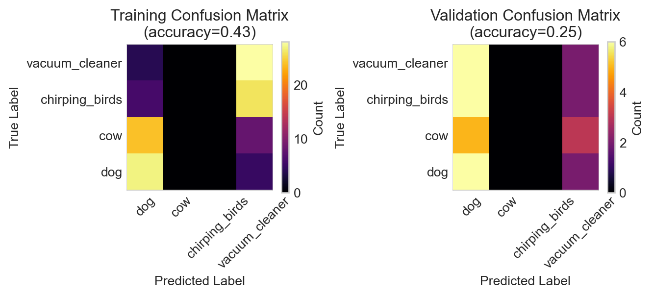
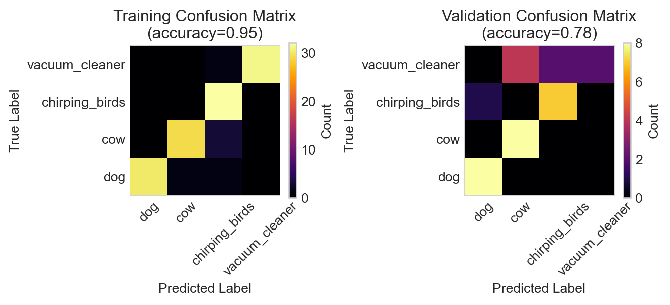
Figure 14.4: Confusion matrices for the RNN model on the training and validation data.

The RNN has badly overfit the training data, achieving high accuracy on the training set but essentially random guessing on the validation data. Although it may be possible to salvage the RNN, let’s instead try a different model architecture and data representation.

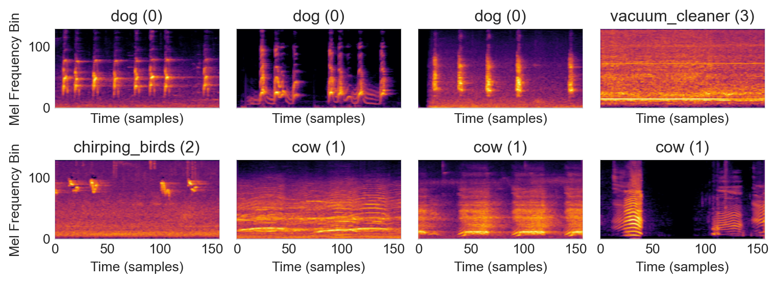
Convolutional Neural Networks for Spectrograms

Since we are already familiar with methods for image data sets, what if we leveraged the image-like structure of spectrograms as a stage in our feature pipeline? We could then use convolutional architectures in the hopes of better performance.

Since we added a transform argument to our WavDataset class, this is as easy as implementing a short function which computes the spectrogram from the input waveform:

def spectrogram_transform(y): 
    mel_spectrogram = librosa.feature.melspectrogram(y=y, sr=16000, n_mels=128, fmax=8000)
    return librosa.power_to_db(mel_spectrogram, ref=np.max)

Now we can pass this transform int othe construction of new data sets:

spectrogram_train_dataset = WavDataset(train_df, "train", transform=spectrogram_transform)
spectrogram_val_dataset   = WavDataset(val_df, "val", transform=spectrogram_transform)

spectrogram_train_loader  = DataLoader(spectrogram_train_dataset, batch_size=8, shuffle=True)
spectrogram_val_loader    = DataLoader(spectrogram_val_dataset, batch_size=8, shuffle=False)

We can check that a batch of the data loader now returns a feature tensor X with three dimensions: (batch_size x height x width).

X, y, labels = next(iter(spectrogram_train_loader))
print(X.shape)

torch.Size([8, 128, 157])

Here’s a visualization of a complete data batch, including the labels:

Code

fig, axarr = plt.subplots(2, 4, figsize=(8, 3), sharex=True, sharey=True)

for i in range(8): 
    axarr.ravel()[i].imshow(X[i].cpu().squeeze(), aspect="auto", origin="lower", zorder = 10, cmap = "inferno")
    axarr.ravel()[i].set_title(f"{labels[i]} ({y[i].item()})")
    axarr.ravel()[i].set_xlabel("Time (samples)")
axarr[0, 0].set_ylabel("Mel Frequency Bin")
axarr[1, 0].set_ylabel("Mel Frequency Bin")
plt.tight_layout()
plt.show()

Figure 14.5: Complete batch of 8 spectrograms queried from `spectrogram_train_loader`.

For our model, we’ll use a simple convolutional architecture in which we stack kernel convolutions, ReLU nonlinearities, and max pooling.

class ConvNet(torch.nn.Module):
    def __init__(self, num_classes):
        super().__init__()
        self.pipeline = torch.nn.Sequential(
            torch.nn.Conv2d(1, 16, kernel_size=3, padding=1),
            torch.nn.ReLU(),
            torch.nn.MaxPool2d(2),
            torch.nn.Conv2d(16, 32, kernel_size=3, padding=1),
            torch.nn.ReLU(),
            torch.nn.MaxPool2d(2),
            torch.nn.Conv2d(32, 64, kernel_size=3, padding=1),
            torch.nn.ReLU(),
            torch.nn.MaxPool2d(2),
            torch.nn.Conv2d(64, 128, kernel_size=3, padding=1),
            torch.nn.ReLU(),
            torch.nn.MaxPool2d(2),
            torch.nn.Flatten(),
            torch.nn.Linear(9216, num_classes)
        )

    def forward(self, x):
        out = x.unsqueeze(1)
        return self.pipeline(out)

model = ConvNet(num_classes=len(CATEGORIES)).to(device)

Perhaps importantly, this model has many fewer parameters than the RNN.

num_params = sum(param.numel() for param in model.parameters())
print(f"Number of parameters in the model: {num_params}")

Number of parameters in the model: 134020

We can get a more detailed view of the model architecture and the shapes of the intermediate outputs using the summary function from the torchinfo package.

X, y = next(iter(spectrogram_train_loader))[:2]
summary(model, input_size=X.shape, device = device)

==========================================================================================
Layer (type:depth-idx)                   Output Shape              Param #
==========================================================================================
ConvNet                                  [8, 4]                    --
├─Sequential: 1-1                        [8, 4]                    --
│    └─Conv2d: 2-1                       [8, 16, 128, 157]         160
│    └─ReLU: 2-2                         [8, 16, 128, 157]         --
│    └─MaxPool2d: 2-3                    [8, 16, 64, 78]           --
│    └─Conv2d: 2-4                       [8, 32, 64, 78]           4,640
│    └─ReLU: 2-5                         [8, 32, 64, 78]           --
│    └─MaxPool2d: 2-6                    [8, 32, 32, 39]           --
│    └─Conv2d: 2-7                       [8, 64, 32, 39]           18,496
│    └─ReLU: 2-8                         [8, 64, 32, 39]           --
│    └─MaxPool2d: 2-9                    [8, 64, 16, 19]           --
│    └─Conv2d: 2-10                      [8, 128, 16, 19]          73,856
│    └─ReLU: 2-11                        [8, 128, 16, 19]          --
│    └─MaxPool2d: 2-12                   [8, 128, 8, 9]            --
│    └─Flatten: 2-13                     [8, 9216]                 --
│    └─Linear: 2-14                      [8, 4]                    36,868
==========================================================================================
Total params: 134,020
Trainable params: 134,020
Non-trainable params: 0
Total mult-adds (M): 575.60
==========================================================================================
Input size (MB): 0.64
Forward/backward pass size (MB): 38.40
Params size (MB): 0.54
Estimated Total Size (MB): 39.58
==========================================================================================

Let’s now run a standard training loop, again using our custom data loaders.

loss_fn = torch.nn.CrossEntropyLoss()
optimizer = torch.optim.Adam(model.parameters(), lr=0.001)

for epoch in range(10):
    model.train()
    for X_batch, y_batch, _ in spectrogram_train_loader:
        optimizer.zero_grad()
        outputs = model(X_batch)
        loss = loss_fn(outputs, y_batch)
        loss.backward()
        optimizer.step()

This model performs much better than the RNN:

Code

acc, loss, cm = evaluate(model, spectrogram_train_loader)
fig, axarr = plt.subplots(1, 2, figsize=(7, 3))
ax = axarr[0]
plot_confusion_matrix(cm, CATEGORIES, ax)
ax.set_title(f"Training Confusion Matrix\n(accuracy={acc:.2f})")

acc, loss, cm = evaluate(model, spectrogram_val_loader)
ax = axarr[1]
plot_confusion_matrix(cm, CATEGORIES, ax)
ax.set_title(f"Validation Confusion Matrix\n(accuracy={acc:.2f})")
plt.tight_layout()

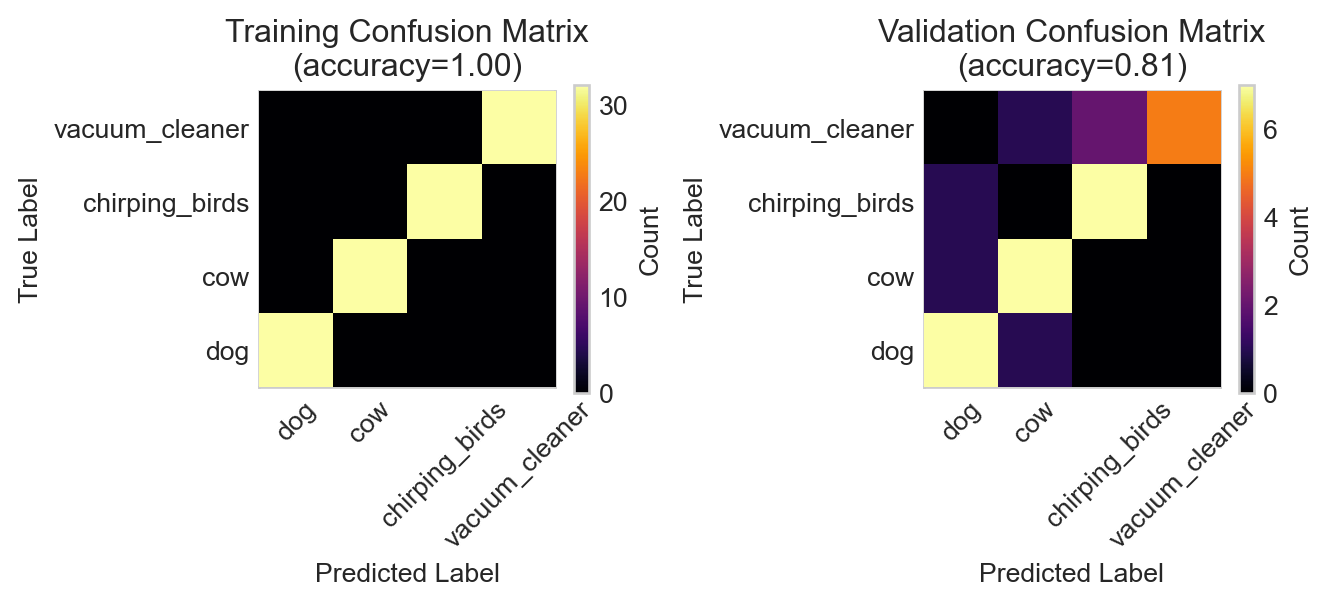
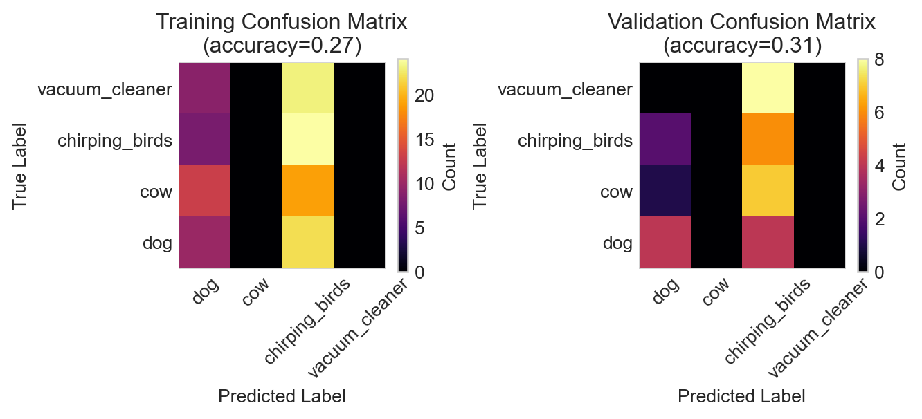
Figure 14.6: Training and validation confusion matrices for the convolutional neural network.

While some evidence of overfitting is present, the convolutional architecture has achieved a much better accuracy on the classification problem than the recurrent architecture.

Data Augmentation

Consider the following example from our training set:

Code

path = "wav_data/train/5-9032-A-0.wav"
audio, sr = librosa.load(path, sr=16000)

spec = spectrogram_transform(audio)

label = metadata[metadata["filename"] == "5-9032-A-0.wav"]["category"].values[0]

fig, ax = plt.subplots(figsize=(7, 3))
im = librosa.display.specshow(spec, y_axis='mel', fmax=8000, x_axis='time', ax = ax)
ax.set_title(f"Mel Spectrogram of {path} ({label})")
t = plt.colorbar(im, label="Magnitude", format='%+2.0f dB')

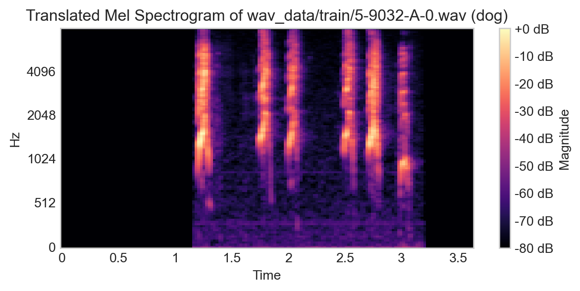
If we were to translate this signal by simply sliding it to the left or right, the appropriate label wouldn’t change, since we’re effectively just adding a time-delay to the recording.

Code

# translate the spectrogram by 10 time steps
translated_spec = np.roll(spec, shift=50, axis=1)
fig, ax = plt.subplots(figsize=(7, 3))
im = librosa.display.specshow(translated_spec, y_axis='mel', fmax=8000, x_axis='time', ax = ax)
ax.set_title(f"Translated Mel Spectrogram of {path} ({label})")
t = plt.colorbar(im, label="Magnitude", format='%+2.0f dB')

This insight implies that we can effectively create new data from our current data simply by applying transformations that preserve the data structure, in this case time-domain translation. Here’s a pipeline which implements this:

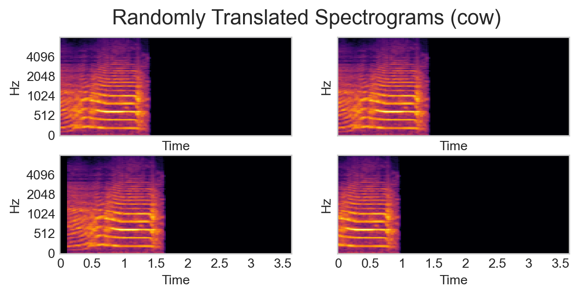
def transform_pipeline(y):
    
    # previous transform to obtain spectrogram
    spec = spectrogram_transform(y)
    
    # randomly translate the spectrogram by up to 20% of its width in either direction and pad with -80 dB (the minimum value in the spectrogram) on the side that gets rolled over
    max_translation_frac = 0.2
    translation_frac = np.random.uniform(0, max_translation_frac)
    pixels_to_translate = int(translation_frac * spec.shape[1])
    pixels_to_translate = np.random.choice([-pixels_to_translate, pixels_to_translate])
    translated_spec = np.roll(spec, shift=pixels_to_translate, axis=1)
    if pixels_to_translate > 0:
        translated_spec[:, :pixels_to_translate] = -80
    else:
        translated_spec[:, pixels_to_translate:] = -80
    return translated_spec

We can now define a new data set and data loader that use this pipeline:

spectrogram_train_dataset_aug = WavDataset(train_df, "train", transform=transform_pipeline)
spectrogram_val_dataset_aug = WavDataset(val_df, "val", transform=transform_pipeline)

spectrogram_train_loader_aug = DataLoader(spectrogram_train_dataset_aug, batch_size=8, shuffle=True)
spectrogram_val_loader_aug = DataLoader(spectrogram_val_dataset_aug, batch_size=8, shuffle=False)

If we now query the data set multiple times, we’ll get slightly different versions of the same spectrogram:

first_query = spectrogram_train_dataset_aug[4][0]
second_query = spectrogram_train_dataset_aug[4][0]

print(torch.all(first_query == second_query))

tensor(False, device='mps:0')

Here are a few examples of queries for the same entry of the data set:

Code

fig, axarr = plt.subplots(2, 2, figsize=(7, 3), sharex=True, sharey=True)

for i, ax in enumerate(axarr.flat):
    spec, label, category = spectrogram_train_dataset_aug[4]
    im = librosa.display.specshow(spec.cpu().numpy(), y_axis='mel', fmax=8000, x_axis='time', ax = ax, cmap = "inferno")

fig.suptitle(f"Randomly Translated Spectrograms ({category})", fontsize=16)

plt.show()

Now let’s try training a model on this new, augmented data set:

loss_fn = torch.nn.CrossEntropyLoss()
optimizer = torch.optim.Adam(model.parameters(), lr=0.001)

for epoch in range(10):
    model.train()
    for X_batch, y_batch, _ in spectrogram_train_loader_aug:
        optimizer.zero_grad()
        outputs = model(X_batch)
        loss = loss_fn(outputs, y_batch)
        loss.backward()
        optimizer.step()

How did we do?

acc, loss, cm = evaluate(model, spectrogram_train_loader_aug)
fig, axarr = plt.subplots(1, 2, figsize=(7, 3))
ax = axarr[0]
plot_confusion_matrix(cm, CATEGORIES, ax)
ax.set_title(f"Training Confusion Matrix\n(accuracy={acc:.2f})")

acc, loss, cm = evaluate(model, spectrogram_val_loader)
ax = axarr[1]
plot_confusion_matrix(cm, CATEGORIES, ax)
ax.set_title(f"Validation Confusion Matrix\n(accuracy={acc:.2f})")
plt.tight_layout()

The use of data augmentation is often a way to reduce overfitting – showing a model multiple randomly perturbed versions of the same data point can allow the model to learn to ignore the random perturbations.

Other Data Augmentation

In our example, random horizontal translation was an appropriate way to augment our data, since this corresponded simply to adjusting the timing of the recording. In other contexts, other kinds of data augmentation may be appropriate. For example, in the context of image classification, random flips and rotations might also be appropriate. For example, all of the following transformed images depict a cat:

Figure 14.8: *Some other kinds of data augmentation for image classification. Image credit: isahit.*

Transfer Learning

Training machine learning models is fun and all, but wouldn’t it be easier if we could have someone else do the hard work for us?

Definition 14.1 (Transfer Learning) Transfer learning is the practice of accessing a model trained on a different-but-related task and retraining it for the desired task.

For example, in our case there are likely no models that are specifically specialized for the four-way classification problem we’ve considered here. However, there are lots of models trained on spectrograms more generally. So, if we accessed a spectrogram model, we could modify and retrain it for our application.

For example, let’s grab a generic trained image classification model. We’ll then “freeze” most of its parameters and train only the final linear layer:

from torchvision import models
model = models.resnet18(weights='IMAGENET1K_V1')
model = model.to(device)
for param in model.parameters():
    param.requires_grad = False
    
model.fc = torch.nn.Linear(512, len(CATEGORIES)).to(device)

This model requires us to pass an image with 3 channels, for which we’ll just duplicate the spectrogram three times:

def transform_pipeline_transfer(y):    
    Y = torch.tensor(transform_pipeline(y))
    return torch.tile(Y, dims = (3, 1, 1))

In principle, we’re now ready to train and evaluate the model:

Code

transfer_dataset_train = WavDataset(train_df, "train", transform=transform_pipeline_transfer)
transfer_dataset_val = WavDataset(val_df, "val", transform=transform_pipeline_transfer)

transfer_loader_train = DataLoader(transfer_dataset_train, batch_size=8, shuffle=True)
transfer_loader_val = DataLoader(transfer_dataset_val, batch_size=8, shuffle=False)

opt = torch.optim.Adam(model.parameters(), lr=1e-3)

for epoch in range(5):
    model.train()
    for X_batch, y_batch, _ in transfer_loader_train:
        optimizer.zero_grad()
        outputs = model(X_batch)
        loss = loss_fn(outputs, y_batch)
        loss.backward()
        optimizer.step()
    
acc, loss, cm = evaluate(model, transfer_loader_train)
fig, axarr = plt.subplots(1, 2, figsize=(7, 3))
ax = axarr[0]
plot_confusion_matrix(cm, CATEGORIES, ax)
ax.set_title(f"Training Confusion Matrix\n(accuracy={acc:.2f})")

acc, loss, cm = evaluate(model, transfer_loader_val)
ax = axarr[1]
plot_confusion_matrix(cm, CATEGORIES, ax)
ax.set_title(f"Validation Confusion Matrix\n(accuracy={acc:.2f})")
plt.tight_layout()

Figure 14.9: Performance of the lightly-retrained ResNet18 model on the audio classification task.

In this particular instance transfer learning has not been more effective than our simple convolutional network. This makes sense because the complexity of the pretrained network is so much higher than the complexity of the data set and task we have given it. It’s also important to note that most images don’t look like spectrograms, so a model trained on generic images may not be as effective here. For a more detailed look at transfer learning for image classificatino tasks, see this tutorial.

References

Piczak, Karol J. 2015. “ESC: Dataset for Environmental Sound Classification.” In Proceedings of the 23rd Annual ACM Conference on Multimedia, 1015–18. Brisbane, Australia: ACM Press. https://doi.org/10.1145/2733373.2806390.