1  Measuring Networks

These lecture notes are based on Chapters 6 and 7 of Newman. They are a short set of highlights, and are not a substitute for actually reading these chapters! There will be content not covered in these notes that you’ll need for homework problems.

1.1 Networks and Matrices

Definition 1.1 (Undirected Graph)

An undirected graph \(G = (N, E)\) is a set of nodes \(N\) and a set of edges \(E\subseteq N\times N\). Each element of \(E\) is an unordered pair of nodes in \(N\). An element of \(E\) can be written \((i,j)\), where \(i, j \in N\). In a simple undirected graph, \(i \neq j\).

When \(i = j\) for some element of \(E\), this is called a self-loop. Simple graphs contain no self-loops.

See Newman 6.2 for discussion of self-loops and other ways graphs can be non-simple.

Matrices are fundamental tools for studying networks. Why is that? The key point is that a graph is a collection of pairwise relationships encoded by \(E\), and matrices are really good for describing pairwise relationships!

The Adjacency Matrix

Easily the most fundamental of the matrices associated to a graph \(G\) is the adjacency matrix

Definition 1.2 (Adjacency Matrix)

The adjacency matrix \(\mathbf{A}\) of a graph \(G = (N,E)\) is an \(n \times n\) matrix, where \(n = \left|N\right|\). Its entries are \[ a_{ij} = \begin{cases} 1 &\quad (i,j) \in E \\ 0 &\quad \mathrm{otherwise.} \end{cases} \]

The reason the adjacency matrix is so important is that it is a lossless representation of the graph structure – given knowledge of \(\mathbf{A}\), you can fully reconstruct the graph. Not all matrices have this property.

Walks

Definition 1.3 A walk of length \(k \geq 2\)* in a graph is a set of edges \((i_1,j_1), (i_2,j_2), \ldots, (i_k,j_k)\) with the property that \(i_\ell = j_{\ell-1}\) for each \(2 \leq \ell \leq k\). We say that this is a walk from \(i_1\) to \(j_k\).

A single edge \((i,j)\) is always considered a walk of length 1 from \(i\) to \(j\).

A question that pops up a lot in network analysis is:

How many walks of length \(k\) exist between nodes \(i\) and \(j\)?

The adjacency matrix gives a concise way to address this question. First, let’s consider \(k = 1\). That’s just the number of edges between nodes \(i\) and \(j\), which is exactly \(a_{ij}\). Said another way,

The \(ij\) th entry of \(\mathbf{A}^1\) counts the number of walks of length \(1\) between nodes \(i\) and \(j\).

This turns out to generalize smoothly by induction.

The \(ij\)-th entry of the matrix \(\mathbf{A}^k\) contains the number of walks of length \(k\) from \(i\) to \(j\).

Here’s a sketch of the proof. Suppose that \(\mathbf{W}(k)\) is a matrix whose entry \(w_{ij}(k)\) contains the number of walks between nodes \(i\) and \(j\) of length \(k\). Then, \(\mathbf{W}(k+1) = \mathbf{W}(k)\mathbf{A}\) has entries \(w_{ij}(k+1)\) containing the number of walks of length \(k+1\). To see this, expand the matrix product:

\[[\mathbf{W}(k)\mathbf{A}]_{ij} = \sum_{\ell \in N}w_{i\ell}(k)a_{\ell j}\;.\]

cf. Newman’s eq. 6.22

Exercise: What’s a very fast argument that this sum does indeed express the number of walks of length \(k+1\) from \(i\) to \(j\)?

Working through this exercise and applying induction, you can see that \(\mathbf{W}(k) = \mathbf{A}^k\), which completes the proof.

A Linear Algebra Interlude

What kind of information does the matrix \(\mathbf{A}\) hold about the graph? Well, one answer is “all of it,” because \(\mathbf{A}\) determines the graph up to permutations of node labels. But there’s a more useful answer as well. When we as about the information contained in a matrix, we often look at the eigenvalues and eigenvectors. The eigenvalues and eigenvectors of the adjacency matrix can contain some useful information about the graph structure. Let’s see an example.

Let

\[ \mathbf{K}_n = \left[\begin{matrix} 0 & 1 & 1 & \cdots & 1 \\ 1 & 0 & 1 & \cdots & 1 \\ 1 & 1 & 0 & \cdots & 1 \\ \vdots & \vdots &\vdots &\ddots & \vdots \\ 1 & 1 & 1 & 0 \cdots & 0 \end{matrix}\right]\;. \]

There are \(n\) rows and \(n\) columns.

The is the adjacency matrix of an n-clique: a graph on \(n\) nodes in which all nodes are connected to each other.

Let’s now consider the matrix \[ \mathbf{A}_{2n} = \left[\begin{matrix} \mathbf{K}_n & \mathbf{I}_n \\ \mathbf{I}_n & \mathbf{K}_n \end{matrix}\right]\;. \]

Here, \(\mathbf{I}_n\) is the \(n\times n\) identity matrix.

Now, \(\mathbf{A}_n\) is the matrix of two cliques that have been “paired”, with each node in one clique connected to exactly one node in the other clique. A small example is shown in Figure 1.1.

Code

library(tidygraph)
library(ggraph)
library(tidyverse)

colors <- c("#f5b895", "#0f4c81")

n <- 5

K <- create_complete(n)

K <- K %>%
    mutate(x = ifelse(row_number() <= 2, 0, 1),
           y = ifelse(row_number() %% 2 == 0, 0, 1))

G <- bind_graphs(K, K) %>%
    mutate(id = row_number()) %>%
    mutate(x = ifelse(id > n, x + 2, x),
                 group = round((row_number() <= n)),
                 group = factor(group)) 

G <- G %>%
    bind_edges(tibble(from = 1:(n), to = 1:(n) + n))

G %>% 
    ggraph() +
    geom_edge_link(start_cap = circle(3, 'mm'),
                   end_cap = circle(4, 'mm'), 
                   alpha = .3) +
    geom_node_point(aes(fill = factor(group),  shape = factor(group)),  size = 10, color = "black") +
    scale_shape_manual(values = c(21, 22)) + 
    scale_fill_manual(values = colors) +
    guides(fill = "none", shape = "none") + 
    theme(aspect.ratio = 1,
            panel.background = element_rect(fill = "white"),
            plot.background = element_rect(fill = "white"))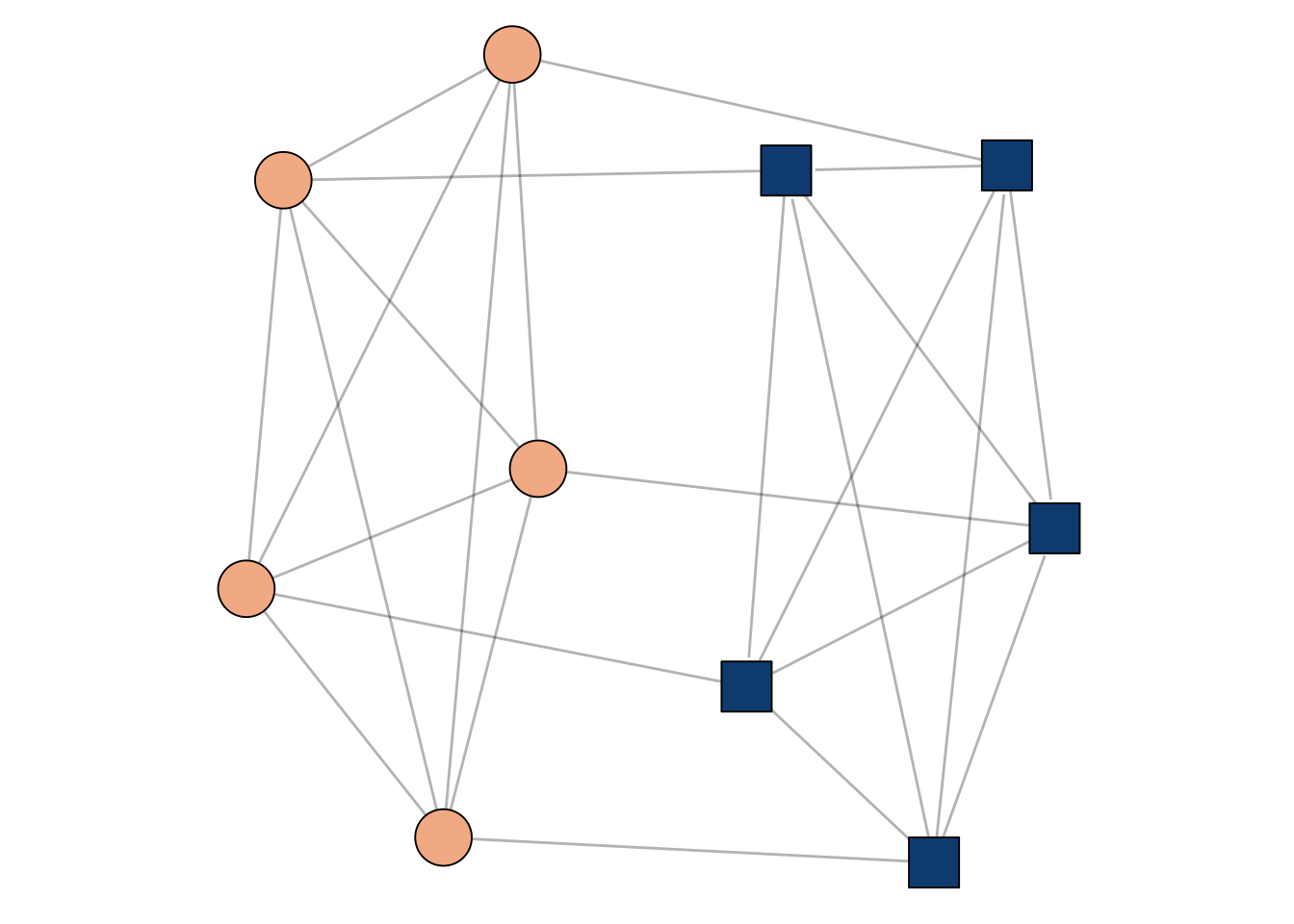 

Figure 1.1: A visualization of the ‘paired cliques’ example with 10 total nodes. Nodes in the first clique are represented by orange circles, and nodes in the second clique by blue squares.

What kinds of information are contained in the first few eigenvectors of \(\mathbf{A}_{2n}\)?

Exercise: The vector of ones \(\mathbf{1}_{2n}\) is an eigenvector of \(\mathbf{A}_{2n}\). What is its eigenvalue? How do we know whether it is the largest one?

Exercise: The vector \(\mathbf{v} = (\mathbf{1}_n, - \mathbf{1}_n)\) is another eigenvector of \(\mathbf{A}_{2n}\). What is its eigenvalue?

In fact, these are the two largest eigenvalues of \(\mathbf{A}\). The first one isn’t very interesting, but note that the second one actually separates the two cliques!

So, suppose we were given a graph where:

• We knew that the graph had the paired-clique structure, but
• We didn’t know which node belonged to which clique.

A way to solve this problem would be to compute the second eigenvector \(\mathbf{v}\). The signs of \(\mathbf{v}\) separate the two cliques. This idea is the foundation of many spectral graph clustering algorithms.

In fact, the adjacency matrix isn’t usually the optimal matrix to use for spectral algorithms. This is a deep and important story related to random matrix theory, which has many connections to network science.

(Nadakuditi and Newman 2012)

Degrees

Definition 1.4 (Degree)

The degree \(k_i\) of a node \(i\) is the number of edges attached to it. \[ k_i = \lvert \left\{j:(i,j) \in E\right\}\rvert\;. \]

The degree is a fundamental quantity in many network analyses. Especially the distribution of degrees in the network can play a major role in both theory and applications.

Exercise: show that the diagonal entries of \(\mathbf{A}^2\) give the degree of each node.

We often collect the degrees into a diagonal matrix \(\mathbf{D}\) whose diagonal entry \(d_{ii} = k_i\) contains the degree of node \(i\).

Exercise: Show that \(\sum_{i = 1}^n d_i = 2m\), where \(m\) is the number of edges in \(G\).

The Laplacian

Another very important matrix for network representations is the graph Laplacian matrix. Actually, there are multiple matrices with claim to this name, but the one we’ll usually focus on is the combinatorial Laplacian.

Definition 1.5 (Combinatorial Graph Laplacian)

The combinatorial Laplacian \(\mathbf{L}\) of a graph with adjacency matrix \(\mathbf{A}\) is \(\mathbf{L} = \mathbf{D} - \mathbf{A}\).

Exercise: Given knowledge of the combinatorial Laplacian \(\mathbf{L}\), is it possible to exactly reconstruct the graph?

The Laplacian is often used to represent (diffusive) flows of quantities between nodes. To see why, suppose that I have some amount of water \(x_i\) on each node \(i\), and that I collect this into a vector \(\mathbf{x}\). Now, consider the vector \(\mathbf{L}\mathbf{x}\).

\[ \begin{align} [\mathbf{L}\mathbf{x}]_i &= \sum_{j} \left(d_{ij}x_j - a_{ij}x_j \right) \\ &= \underbrace{k_ix_i}_{\text{flow out of }i} - \underbrace{\sum_{j} a_{ij}x_j}_{\text{flow into }i}\;. \end{align} \]

The first term distributes the water \(x_i\) at node \(i\) to each of \(i\)’s \(k_i\) neighbors, while the second term allows water to flow into node \(i\) from each neighbor along each edge connecting them.

The Laplacian matrix \(\mathbf{L}\) will appear in several places throughout this course, when we consider random walks, graph partitioning, and dynamical systems.

Many More Matrices…

There are LOTS of matrices that can be associated to networks. There’s no “right” one – some are more useful than others for certain jobs. Throughout this course, we’ll see examples of matrices that are well-suited to certain specific tasks, like ranking or clustering. If you’re interested in searching around a bit, some other fun matrices are:

• The nonbacktracking or Hashimoto matrix.
• The modularity matrix.
• The random-walk transition matrix.
• The random-walk and symmetric normalized Laplacian matrices.
• The PageRank matrix.
• The node-edge incidence matrix.

And the list goes on!

Directed and Weighted Graphs

Newman Chapter 6 contains a nice introductory discussion of directed and weighted graphs. We won’t spend a lot of time on these at this stage of the course, but it’s worthwhile reading this material as it may be of interest as you think about projects.

Measures and Metrics

There are lots of questions we can ask about network data. Even in the setting of simple graphs, there are some very interesting questions with surprisingly complex answers. In this section, we’ll consider some (not all) of the most important things to measure in networks.

Ideas Connected to Walks

Walks are a fundamental idea in networks. If we imagine networks as connecting things together, walks and walk counts are direct quantifications of how “connected” the network really is. Here are a few things we can measure about networks using walks.

Connected Components

Definition 1.6 (Connected Components)

Two nodes \(i\) and \(j\) are path-connected if there exists a path \(i \leftrightarrow j\). The set of nodes \(j\) such that \(i\) is path-connected to \(j\) is called the connected component of \(i\). A network is connected if it has only one connected component.

Exercise: Show that the relation “\(i\) is path-connected to \(j\)” is an equivalence relation on the set of nodes \(N\).

Intuitively, a disconnected network is fragmented into two or more pieces. Almost all network analysis problems are most interesting and challenging when the network is connected, and so we’ll often assume this in data analysis applications. Mathematically, however, the question of when certain models of networks become connected has a very rich theory that we’ll see a small part of.

Geodesics and Graph Diameter

Definition 1.7 (Geodesic Paths)

The length of a walk is the number of edges it contains. A geodesic path (also called a shortest path) from \(i\) to \(j\) is a walk fom \(i\) to \(j\) of minimum length; i.e. a walk such that no other walk has shorter length. The length of a geodesic path is called the (geodeisc) distance between \(i\) and \(j\). If two nodes are not path-connected, their geodesic distance is undefined.

Code

library(tidygraph)
library(igraph)
library(ggraph)

set.seed(1234)

g <- erdos.renyi.game(20, 40, type = "gnm") %>%
    as_tbl_graph()

path <- shortest_paths(g, 5, 12)$vpath

E(g, path=path[[1]])$on_path <- TRUE

g <- g %>% 
    as_tbl_graph() %>% 
    activate(edges) %>% 
    mutate(on_path = !is.na(on_path))

g %>% 
  ggraph() + 
  geom_edge_link(aes(width = on_path), alpha = 0.7) + 
  geom_node_point(size = 7, pch = 21, fill = "#73b9ee") + 
  theme_void() + 
  scale_edge_width_manual(values = c(.3, 2)) +  
  guides(edge_color = "none", edge_width = "none")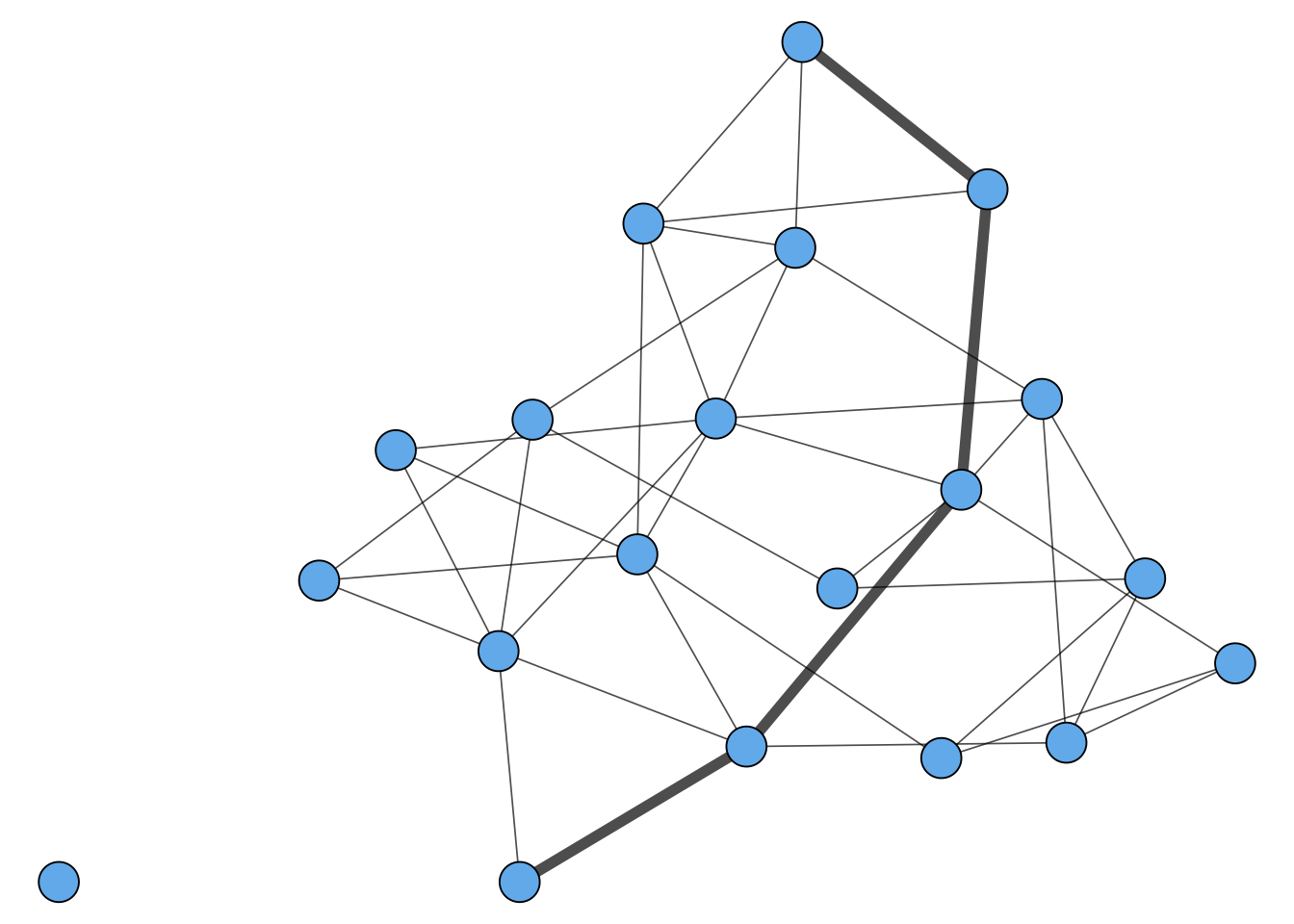

A graph with 20 nodes and 40 edges. While it can be difficult to navigate through even small graphs, note that some nodes are clearly close together, while others are far apart.

A geodesic (shortest path) is shown between two selected nodes.

There is one node that is not connected to any of its neighbors, and its distance to them is undefined. As a result, this graph has undefined diameter.

The diameter of a graph is the longest length of geodesic paths across all pairs of nodes. If the graph is disconnected, the diameter is undefined.

Another way to say this is that, in a connected graph, the diameter is the distance between the two nodes that are farthest away.

Betweenness Centrality

How important is a node? We’ll come back to this question several times in the course. The idea of geodesic paths allows us to consider one approach to this question:

Idea: A node is important if you frequently have to go through it to get to other nodes.

This idea leads us to the idea of betweenness centrality.

Definition 1.8 (Betweenness Centrality)

The betweenness centrality \(b_i\) of a node \(i\) is the number of geodesic paths in the graph that pass through node \(i\).

Figure 1.2 shows a network with nodes sized according to their betweenness centrality.

Code

library(tidygraph)
library(ggraph)
library(igraph)
library(tidyverse)
library(igraphdata)
data(karate)

g <- karate %>% 
    as_tbl_graph() %>% 
    mutate(btwn = centrality_betweenness())

g %>% 
    ggraph() +
    geom_edge_link(alpha = 0.2) + 
    geom_node_point(aes(size = btwn), pch = 21, fill = "#73b9ee") + 
    theme_void() + 
    guides(size = "none") + 
    scale_size_continuous(range = c(3, 15))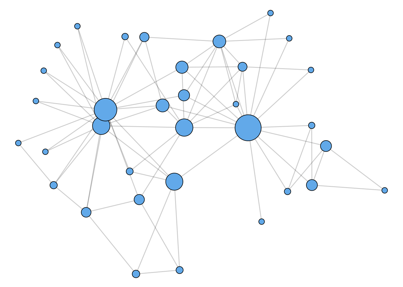

Figure 1.2: The famous Zachary Karate Club network (Zachary 1977). The size of each node reflects its betweenness centrality.

Katz Centrality

Here’s another centrality concept that is going to draw on our linear algebra skills a bit.

Recall that \(\mathbf{A}^k\) has entries that count the total number of walks of length \(k\) between two nodes. Here’s an alternative idea of node importance:

A node \(i\) is important when there are lots of short walks in the graph that lead to \(i\).

This idea takes a bit more effort to operationalize mathematically.

First, the number of walks of length \(k\) that lead to each node can be computed by the vector \(\mathbf{v}(k) = \mathbf{A}^k\mathbf{1}_n\). Now, \(v_i(k)\) gives the total number of \(k\)-walks that lead to node \(i\). Now, the total number of walks of length \(\ell\) or less leading to \(i\) is \(\sum_{k = 1}^{\ell} v_i(k)\).

Now, if we all \(\ell \rightarrow \infty\), then we’ll find that the total number of walks to \(i\) is infinite. But we can make progress if we instead decide that short walks are more important than longer walks. This makes sense – if I have to go on a long walk to find you, then you might be in a relatively remote, out-of-the-way location.

So, we’ll add a discount factor \(\alpha < 1\). A walk of length \(k\) gets a discount of \(\alpha^k\). The weighted number of walks to \(i\) is \(\sum_{k = 1}^{\infty} \alpha^kv_i(k)\). The vector containing this information for each node is the vector

\[ \mathbf{v}(\alpha) = \sum_{k = 1}^{\infty} \alpha^k\mathbf{v}(k)\;. \]

Perhaps surprisingly, we’re not stuck. Recall the definition of \(\mathbf{v}(k)\), which lets us write

\[ \mathbf{v}(\alpha) = \sum_{k = 1}^{\infty} \alpha^k\mathbf{A}^k\mathbf{1}_n = \left[\sum_{k = 1}^{\infty} (\alpha\mathbf{A})^k\right]\mathbf{1}_n\;. \]

Now we need a matrix trick.

If \(\mathbf{B}\in \mathbb{R}^{n\times n}\) is a symmetric matrix and \(\left|\lambda\right| < 1\) for any eigenvalue \(\lambda\) of \(\mathbf{B}\), then
\[ \sum_{k = 1}^{\infty} \mathbf{B}^k = (\mathbf{I}_n - \mathbf{B})^{-1} - \mathbf{I}_n\;. \]

Compare this theorem to the geometric series formula \[ \sum_{k = 1}^{\infty} r^k = (1 - r)^{-1} - 1 \] for scalar \(\left|r \right| < 1\).

We can use this result to compute \(\mathbf{v}(\alpha)\). Provided that \(\alpha\) is smaller than \(\frac{1}{\left|\lambda\right|}\) for any eigenvalue \(\lambda\) of \(\mathbf{A}\), we have the Katz centrality.

Definition 1.9

The Katz centrality (Katz 1953) of node \(i\) with parameter \(\alpha\) is the \(i\)th entry of the vector \[ \mathbf{v}(\alpha) = ((\mathbf{I}_n - \alpha\mathbf{A})^{-1} - \mathbf{I}_n)\mathbf{1}_n\;. \]

Code

library(tidygraph)
library(ggraph)
library(igraph)
library(tidyverse)
library(igraphdata)
data(karate)

g <- karate %>% 
    as_tbl_graph() %>% 
    mutate(btwn = centrality_katz(alpha = .05))

g %>% 
    ggraph() +
    geom_edge_link(alpha = 0.2) + 
    geom_node_point(aes(size = btwn), pch = 21, fill = "#73b9ee") + 
    theme_void() + 
    guides(size = "none") + 
    scale_size_continuous(range = c(3, 15))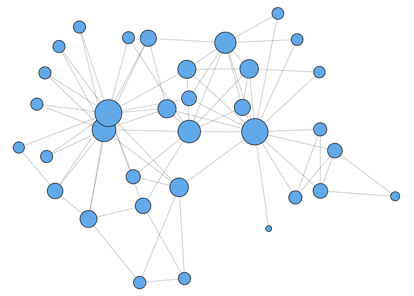

Figure 1.3: The Zachary Karate Club network (Zachary 1977). The size of each node reflects its Katz centrality with α = 0.05.

As shown in Figure 1.3, the Katz centrality leads to less dramatic results, while still highlighting nodes that appear to be “in the center” of the graph.

Triadic Closure (Transitivity)

Think of two of your friends. Are they friends with each other? This kind of “coincidence” happens quite frequently in social networks. Let’s look at two ways to quantify this effect.

In graph terms, when you think of two of your friends, you are thinking of two edges connected to you in your social network, and asking whether there exists a third edge that creates a triangle. So, we have a situation like that shown in Figure 1.4.

Code

library(ggraph)
library(tidyverse)
library(tidygraph)

tbl_graph(
    edges = tibble(
        from = c(1, 1, 3), 
        to = c(2, 3, 2),
        q = c(FALSE, FALSE, TRUE)
        )
    ) %>% 
    ggraph() + 
    geom_edge_link(aes(edge_linetype = q), alpha = 0.6, edge_width = 3) + 
    geom_node_point(pch = 21, fill = "#73b9ee", size = 15) + 
    theme_void() + 
    guides(edge_linetype = "none")

Figure 1.4: Triadic closure. The two solid edge form a wedge (a possible triangle). The dashed edge turns the wedge into a (realized) triangle.

When the dotted line “closes the triangle,” we often call this “closing the triangle.* The phrase triadic closure, also sometimes called transitivity, refers to the existence of large numbers of closed triangles in many social networks.

How do we quantify triadic closure? There’s a simple approach to this:

Definition 1.10 (Local Clustering) The local clustering coefficient \(C_i\) measures the proportion of possible triangles connected to \(i\) that are realized. If \(i \sim j\) means “\(i\) and \(j\) are connected, then we can write this as

\[ C_i = \frac{\sum_{j, \ell \sim i} a_{j\ell}}{\binom{k_i}{2}} \]

Remember: \(k_i\) is the degree (number of neighbors) of node \(i\).

In this definition, the denominator is the number of pairs of neighbors of node \(i\). We can think of this as counting the number of possible triangles. The numerator is then the number of realized triangles. The local clustering coefficient is always a number between 0 and 1.

Exercise: Write the numerator in terms of the adjacency matrix \(\mathbf{A}\).

Hint: a triangle is a special kind of walk of length \(3\).

The local clustering coefficient tells us about the rate of triadic closure around a specific node \(i\). There is also a global clustering coefficient that quantifies the rate of triadic closure in the entire network. The idea is the same: it’s the proportion of possible triangles that are actualized:

Definition 1.11 (Global Clustering)

The global clustering coefficient of a graph is \[ \frac{\text{Number of triangles} \times 3}{\text{Number of wedges}} \] Here, a wedge is a possible triangle, like the solid lines shown in the figure above.

The reason for the factor of 3 in the numerator is that the same triangle can be formed from 3 different wedges.

cf. Newman p. 184

It is not the case that the global clustering coefficient can be obtained by averaging the local clustering coefficients!

The prevalence of triadic closure in many real-world networks motivated one of the first mega-papers in network science, which proposed a mathematical model of networks that included clustering (Watts and Strogatz 1998). A sample from this model is shown in Figure 1.5. This paper has now been cited 48,000 times over 24 years.

Code

library(igraph)
library(ggraph)

g <- sample_smallworld(1, 20, 3, 0.05)

g %>% 
    ggraph() +
    geom_edge_link(alpha = 0.2) + 
    geom_node_point(pch = 21, fill = "#73b9ee", size = 6) + 
    theme_void() + 
    guides(size = "none")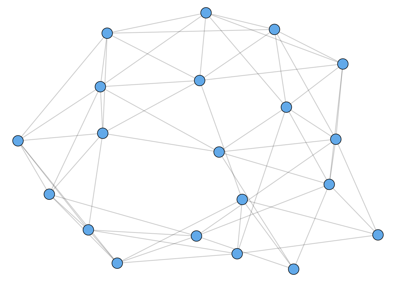

Figure 1.5: A small network sampled from the small-world model of Watts and Strogatz (1998). This model generates graphs with high clustering coefficients. You can likely pick out a large number of triangles by eye.

Community Structure and Graph Cuts

Many networks display what is sometimes called community structure. There isn’t really a formal definition of community structure, but it refers broadly to the idea that a graph can often be divided into multiple parts. Here’s an example of a graph with community structure:

Code

# R code
library(tidygraph)
library(ggraph)

set.seed(1234)

g <- play_islands(2, 10, 0.7, 2)

g %>% 
  ggraph() + 
  geom_edge_link(alpha = 0.5) + 
  geom_node_point(size = 7, pch = 21, fill = "#73b9ee", color = "black") + 
  theme_void()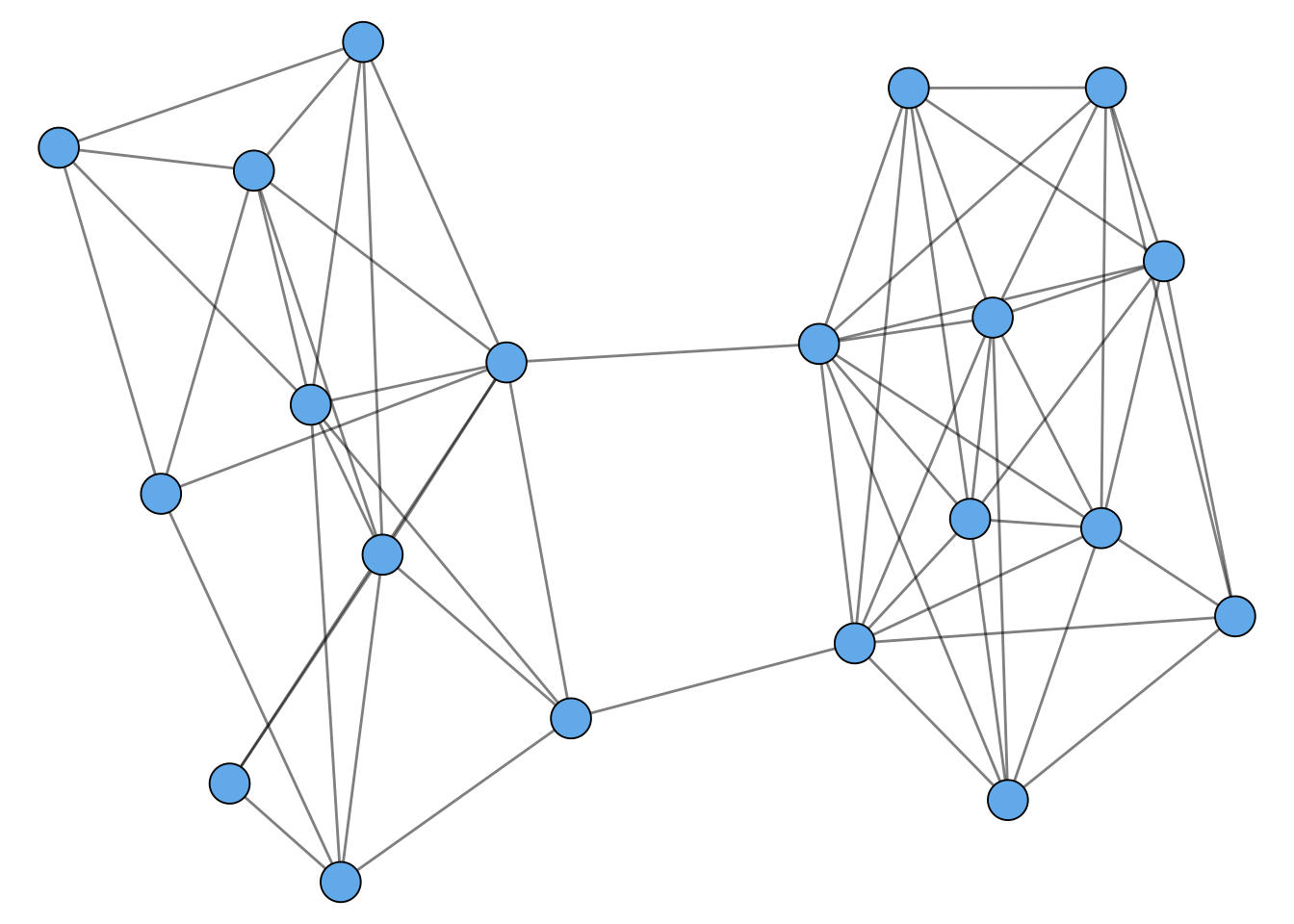

A network with 20 nodes. This network displays one of many common properties in real-world networks, called community structure. In this case, the network is clustered into two densely interconnected ‘communities’ that are only loosely connected to each other. Community structure often accompanies phenomena such as echo chambers in online media.

You might be able to visually separate this graph into two pieces. Heuristically, what we’re looking for is lots of edges within each piece, but few edges between the pieces.

Let’s formalize this a bit.

Definition 1.12 (Clustering) A clustering \((C_1,\ldots,C_\ell)\) of a graph is a partition of the nodes:

\[ N = \bigcup_{j = 1}^{\ell} C_j\;, \quad C_j \cap C_{j'} = \emptyset\;. \]

We’ll write the cluster holding node \(i\) as \(c_i\).

Note: “clustering” here is confusingly and totally unrelated to the “clustering coefficients” from before.

Definition 1.13 (Cut Size) The cut size of a clustering is the number of edges that connect nodes in different clusters:

\[ \mathrm{Cut}(C_1,\ldots,C_\ell) = \frac{1}{2}\sum_{i \neq j} a_{ij}\mathbb{1}[c_i \neq c_j] \]

The reason for the factor \(1/2\) is that we don’t need to count the edges \((i,j)\) and \((j,i)\) separately – it’s the same edge!

An important special case arises when we aim to partition a graph into two clusters. In this case, we can write the cut size in terms of our friend, the combinatorial graph Laplacian.

Let \(\mathbf{s} \in \mathbb{R}^n\) be the vector with entries

\[ s_i = \begin{cases}+1 &\quad i \in C_1 \\ -1 &\quad i \in C_2\end{cases}\;. \]

Theorem 1.1 (Laplacian Formula for Cuts)

We have \(\mathrm{Cut}(C_1,C_2) = \frac{1}{4}\mathbf{s}^T\mathbf{L}\mathbf{s}\).

Proof. To prove this, let’s start by just computing \(\mathbf{x}^T\mathbf{L}\mathbf{x}\) for arbitrary \(\mathbf{x} \in \mathbb{R}^n\). We need to recall the definition of \(\mathbf{L}\) from Definition 1.5. We have \[ \begin{aligned} \mathbf{x}^T\mathbf{L}\mathbf{x} &= \mathbf{x}^T(\mathbf{D} - \mathbf{A})\mathbf{x} \\ &= \mathbf{x}^T\mathbf{D}\mathbf{x}^T - \mathbf{x}^T\mathbf{A}\mathbf{x} \\ &= \sum_{i\in N} k_{i} x_i^2 - \sum_{i,j \in N} a_{ij}x_ix_j \\ &= \frac{1}{2}\left(\sum_{i\in N} k_{i} x_i^2 - 2\sum_{i,j \in N} a_{ij}x_ix_j - \sum_{j\in N} k_{j} x_j^2\right) \\ &= \frac{1}{2}\left(\sum_{i,j\in N} a_{ij} x_i^2 - 2\sum_{i,j \in N} a_{ij}x_ix_j - \sum_{i,j\in N} a_{ij} x_j^2\right) \\ &= \frac{1}{2}\sum_{i,j \in N}a_{ij}(x_i - x_j)^2\;. \end{aligned} \]

Let’s use this formula to evaluate \(\mathbf{s}^T\mathbf{L}\mathbf{s}\):

\[ \begin{aligned} \mathbf{s}^T\mathbf{L}\mathbf{s} &= \sum_{i,j \in N}a_{ij}(s_i - s_j)^2 \\ &= \sum_{i,j \in N}a_{ij}(s_i - s_j)^2 \\ &= 4 \sum_{i,j \in N}a_{ij}\mathbb{1}[c_i \neq c_j]\;. \end{aligned} \]

In that last line, we’ve used the fact that \[ (s_i - s_j)^2 = \begin{cases} 2^2 &\quad c_i \neq c_j \\ 0 &\quad \text{otherwise} \end{cases} \quad = \mathbb{1}[c_i \neq c_j]\;. \]

So, we’re done!

Looking Ahead

An important question to ask about many of these metrics is:

What counts as a large, surprising, or meaningful value of a given metric?

One way to address this question is to take some value and compare it to one that we believe to be small, unsurprising, or not meaningful. We often operationalize this by saying that “a random graph” would have some property, such as a low clustering coefficient. So, a high clustering coefficient is surprising, and suggests that the graph might not be “random.” This motivation takes directly to the study of random graphs, which is one of the mathematical foundations of network science.